WD Renner, et. al., "A dose delivery verification method for conventional and intensity-modulated radiation therapy using measured field fluence distributions", Medical Physics, Vol. 30 No. 11, Nov. 2003, pages 2996-3005.

WD Renner, K Norton, T Holmes, "A method for deconvolution of integrated electronic portal images to obtain incident fluence for dose reconstruction", JACMP, Vol. 6, No. 4, Fall 2005, pp. 22-39.

WD Renner, "3D Dose Reconstruction to Insure Correct External Beam Treatment of Patients", Medical Dosimetry, Fall 2007, Vol. 32, No. 3, pages 157-165.

Markus Wendling, Robert J. W. Louwe, Leah N. McDermott, Jan-Jakob Sonke, Marcel van Herk, and Ben J. Mijnheer. Accurate two-dimensional IMRT verification using a back-projection EPID dosimetry method. Med. Phys. 2006;33:259-273.

Anton Mans, Peter Remeijer, Igor Olaciregui-Ruiz, Markus Wendling 1, Jan-Jakob Sonke, Ben Mijnheer, Marcel van Herk, Joep C. Stroom. 3D Dosimetric verification of volumetric-modulated arc therapy by portal dosimetry. Radiotherapy and Oncology 94 (2010) 181–187.

William Swindell, Phillip M. Evans. Scattered radiation in portal images: A Monte Carlo simulation and a simple physical model. Medical Physics, 1996;23(1):63-73.

Methodology:

Steciw, Warkentin, Rathee, and Fallone, reference (1), did a Monte Carlo simulation of the EPID and found that the point spread response of the EPID could be modeled as a sum of five exponentials:

Equation (1)

where n = 5, r is the radius in centimeters.

In Renner et. al. reference (2) we used this model for the point spread of the EPID and devised a way to fit the parameters a_i and b_i. By fitting the parameters we can account for any differences in individual EPIDs and normalize the parameters to produce values from which the dose in centiGray can be computed in a patient.

Given the point spread we can do a deconvolution of an EPID image to transform it back to in air x-ray intensity fluence. This is done by taking the two dimensional transform of the image and dividing each frequency component by the inverse of the transform of the point spread function. The EPID image I_EPID is given by the convolution of the in air x-ray intensity fluence I_fluence that we wish to recover with the point spread function of the EPID:

Equation (2)

where k(r) is the circularly symmetrical point spread of the EPID given by equation (1) above and the symbol designates convolution. Using the convolution theorem, the convolution is the inverse Fourier transform of the multiplication of the Fourier transforms of the image and point spread function respectively:

Equation (3)

If then we break out the I_EPID image in frequency space and divide by F(k(r)), we will in theory recover I_fluence:

Equations (4)

provided F(k(r)) = K(q) below is never zero. In reality, the convolution of the fluence image I_fluence with the point spread in equation (3) above is a low pass spatial frequency operation and spatial frequencies of the fluence image attenuated to noise level amplitudes and lower cannot be recovered.

Using circular symmetry of the EPID point spread, we can use instead the one dimensional Hankel transform of the point spread function instead of a two dimensional Fourier transform for the mathematical convenience of having a closed form transform of k(r) given by K(q) where q is the spatial frequency in cm^-1 and whose value is never zero:

Equation (5)

In the case of recording an EPID exit-transit dose image, there is in addition scatter from the patient that reaches the EPID. This scatter contribution is a further low pass spatial frequency operation. With spatial frequencies of the input fluence attenuated to noise levels and lower, the input fluence image cannot be fully recovered. However, it has been shown that enough can be recovered to give reasonable accuracy in reconstructing the dose the patient receives^3,4.

An additional problem with exit transit images is that the EPID has a strong response dependence upon the input energy of the x-rays. Attenuation by the patient changes the spectrum hitting the EPID and the scatter radiation adds low energy x-rays to the spectrum. Modeling these effects from first principles can be very difficult^3,4. Therefore we continue our point spread fitting procedure to fit a point spread for a series of different thicknesses of water phantom between the EPID and the source of x-rays. This was initially done in 5 cm increments from 0 to 60 cm. Zero thickness corresponds to the prior use of the point spread to recover the input x-ray intensity fluence from the EPID image for pre-treatment dose reconstruction². Fitting a point spread for each thickness for a range of phantom thicknesses produces a series of point spread functions which are indexed by thickness. Between the measured thicknesses the point spread can be interpolated. The end result is a two dimensional point spread that is a function of radius r and thickness th, k(r,th), or in the spatial frequency domain K(q,th), with the kernel for each thickness given by equation (5) above. The number of parameters to fit is now the number of thicknesses times 10 (two for each exponential), but the fitting is done one thickness at a time and is simply a repetition of the fitting procedure used previously for zero thickness.

The point spread of the EPID will include effects of the distance from the phantom to the EPID. However, we will fix the EPID at a constant distance and measure the images with isocenter always in the center of the intervening phantom. The geometry used satisfies the equation:

Air gap = EPID SID cm – (100 cm + ½ water thickness)

and is the nominal geometry assumed for applying the air gap correction below. The EPID SID is to be held at a constant distance for all the images integrated for the EPID kernel.

This will approximate the clinical situation during patient treatment and we can accept errors from not using a more rigorous treatment of exit surface to EPID distance. Any variation of the EPID distance from that which the data is measured for fitting the kernels will result in small errors for small changes in that distance. The error will result from a different scatter contribution from the patient at different EPID distances⁵, not from the inverse square law which is otherwise accounted for, and from the energy sensitivity of the EPID to the scatter radiation. As shown in the below table, the dose at the EPID is insensitive to the air gap distance. Changes due to the air gap are corrected later below.

For a 30 cm thick phantom at 85 cm SSD, 10x10 cm field size we have the following data (data courtesy of Sankar Andiappa, Edinburth, UK):

EPID air

SID gap 6x 10x

________________________________________

140 25 105.7 106.7

145 30 103.8 104.0

150 35 102.3 102.5

155 40 100.1 101.0

160 45 100.0 100.0

165 50 99.3 99.0

170 55 98.7 98.2

175 60 99.0 97.5

180 65 98.8 97.3

where the only the inverse square law has been applied to the EPID signal value on the central axis. If we take our EPID data at 160 cm SID, which is a 45 cm air gap, we see that the error will be 2% for an air gap of 35 cm to 55 cm. The error increases to 6% at an air gap of 25 cm. This dependency will get worst for larger field sizes. But because beams are generally directed at the patient from many angles, will average out to the idea geometry, provided a long EPID distance is maintained. However, we have developed a means to correct for changes in air gap from the above nominal geometry, which will be discussed below.

In all cases, the EPID images are normalized to a calibration field, typically 10x10 cm in field size, for a known monitor unit, typically 100 monitor units, exposed with no intervening phantom, same as doing a pre-treatment case. Therefore the EPID images with different thicknesses has recorded the effect of attenuation by the phantom/patient, scatter from the phantom/patient, beam hardening by the phantom/patient, and energy response of the EPID to the radiation that arrives at the EPID. The point spread is fitted so that the deconvolution process produces the in air x-ray intensity fluence in the units of rmu (relative monitor units), that is, each pixel is normalized to the monitor units required for the calibration field that will produce the same field intensity on the central axis of the calibration field. For open square fields the rmu is the scatter collimator factor times the monitor unit, and otherwise can be thought of as the product of the effective collimator scatter factor times the effective monitor unit.

The deconvolution kernel for each thickness will convert the measured EPID image at each thickness back to the in air x-ray intensity fluence in the units of rmu. The problem remains that for a treatment field on a patient the patient is not a constant uniform thickness presenting a flat surface perpendicular to the central ray of the field. For each pixel on the EPID, we can ray trace the equivalent water thickness that a ray from the source of x-rays transverses to reach that pixel. This will require the plan CT scan set and knowledge of the beam geometry relative to the patient which is obtained from the treatment plan downloaded in Dicom RT format. This ray trace is actually done every fifth pixel with the intervening distances interpolated to save a factor of 25 (5 squared using two dimensional interpolation) in computer time. Using the map of thicknesses now assigned to each pixel in the EPID image, we can now, in theory at least, accomplish a deconvolution for the image by applying the appropriated kernel value at each pixel, indexed by the thickness transversed to reach that pixel by interpolating between the kernels we have for the range of phantom thicknesses.

Such a kernel is a variant kernel and the convolution theorem which would otherwise allow this calculation to be performed in the spatial frequency domain no longer applies. Therefore the deconvolution cannot be performed by multiplication in the frequency domain enabled by use of the Fast Fourier Transform to save computer time, but would have to be performed in the spatial domain. The deconvolution in the spatial domain would have to be with the inverse Fourier Transform of 1/K(q,th).

Performing the deconvolution in the spatial domain with a variant kernel required 9 minutes of time on a 1.81 Giga Hertz Intel based PC running Windows XP. This would mean that a 7 field IMRT case would require an hour of computational time and a IMAT case with an image measured every 5 degrees for a total of 72 images would require close to 11 hours of computation time. These times would be excessive and impractical for clinical use.

The exit images after normalization to the calibration image are reduced to a pixel size of 1 mm, which still leaves us with a 400 x 300 image size for the Varian EPID. We do not want to lose the advantage of the high resolution in using EPID images with any lower resolution although one millimeter is still small compare to the typical pencil sizes of 2 to 5 mm employed.

A one dimensional convolution is of order n squared, whereas the Fast Fourier Transform is of order n log₂ n. These orders are squared for two dimensional images. For a 512 by 512 array size, using the Fast Fourier Transform should be about 3236/2 (division by two for transforming each way) times faster than a discrete convolution. The large computational time required for a discrete deconvolution was eliminated by use of the following approximation. Assume m total thicknesses measured with the EPID resulting in m deconvolution kernels, indexed by the thickness. For a single exit image, deconvolve the image m times for each of the m kernels using the Fast Fourier Transform to produce m intermediate output images. One can use less than the available kernels if the maximum thickness transversed for an image is less than maximum thickness kernel, i.e., if the maximum thickness was 42 cm, then deconvolve using thicknesses 0 to the next thickness larger than 42 cm in that case. Then for each pixel, interpolate between the respective output images to produce a final image. For example, if the thickness transversed for a particular pixel were to be 32.0 cm, then interpolate between the output images deconvolved with the bracketing thicknesses, such as the 30.0 cm thickness kernel and the 35.0 cm thickness kernel if they are the nearest. As the EPID point spread decreases rapidly with radius, and the thickness will usually be slowly varying over the area of the image, this method can be expected to be a reasonable approximation.

Using this scheme, the time required to process the in air fluence image was reduced from 9 minutes to about 1.7 seconds on the same computer with an additional 1.34 seconds needed for the ray trace, for a total of 3.0 seconds per image. On a 2.67 Giga Hertz I7 running under Windows Vista the computer time is about 0.70 seconds per image for the deconvolution process and 0.55 seconds for the ray trace for a total of 1.25 seconds per image. The ray trace is done on a 0.5 cm grid with values interpolated in between nodes.

Transmission through the patient

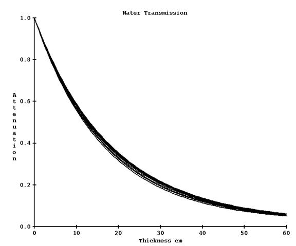
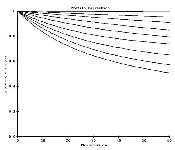
The spectrum of a medical linear accelerator changes off axis and rays off axis are less penetrating the further one goes off axis. To make a correction for this, narrow beam attenuation is measured in steps along the diagonal through a water phantom for a range of water thicknesses. For each ray, the data is fitted to a sum of exponentials for the purpose of interpolation and extrapolation along each ray, with interpolation performed between measured rays. In the process described above, the pixels values can be first corrected for the attenuation by the phantom/patient from the known distance transversed through the phantom/patient. This was implemented as an optional correction. The kernels are fitted either with or without this additional data and can only be used accordingly. However greater accuracy is achieved by first removing the modification the patient caused in the exit image by attenuation by the patient which would change the spatial frequency spectrum of the exit image. Removing that affect before frequency filtering gives more accurate results.

The change in transmission going off axis is not large. Below is a graph of the curves out to a radius of 18 cm for 6x. One could measure only on the central axis and rely on the below profile correction for further refinement of the results.

Scatter from the patient

In the above algorithm we are implicitly making the assumption that the scatter from the phantom/patient is uniform across the EPID. However, this is not entirely true. From reference (5) Figure 4 page 66, for an approximate 14.1x14.1 cm field size the scatter at the central axis is 0.07% of the primary, tapering off to about 0.04% at a radius of 20 cm, at 160 cm distance from the x-ray source for a 20 cm thick water phantom centered at isocenter.

Limitations

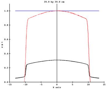
For larger field sizes and thicker phantoms this effect becomes more pronounced. In addition, the EPID will over respond to the scatter radiation. In the below plot we have a profile measured in air with an ion chamber with build up, at a distance of 150 cm from the source of x-rays. At 85 cm SSD is 30 cm of water. The black plot is the ion chamber data scanned for both axes. The red plot is the profile off the EPID image after normalization, and the green plot is after a deconvolution with the EPID point response. Clinical fields are generally not large open fields, so this is not a large issue.

CompareEPIDIonChamber

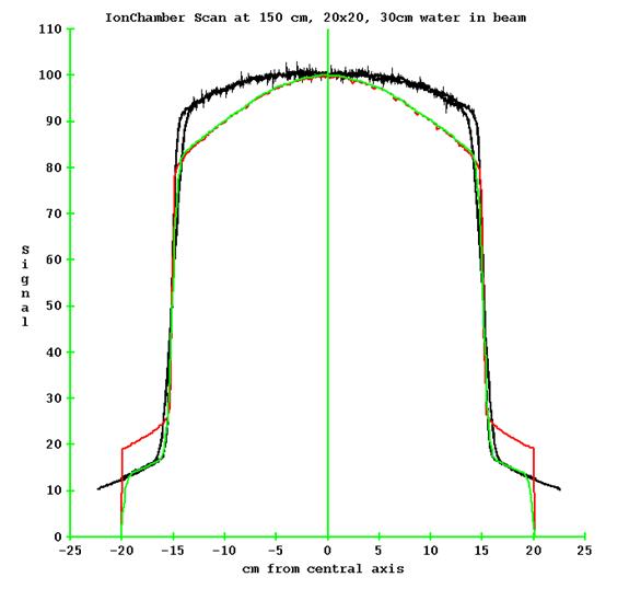
Data courtesy of Muffin Sewell of Vantage Oncology, USA.

Mitigation for large fields at large thicknesses

As of April 2018, this issue was mitigated by fitting the narrow beam off axis transmission after deconvolution to correct for the slope and adding the fit parameters to the EPID kernel file.

In February of 2021 this was modified to leaving the narrow beam transmission data as measured and creating a correction to be applied to the profiles after the frequency filtering of the images. The correction curves are show below for 6x where profiles are to be divided by the correction indexed by radius and thickness. The curves descend more as the radius increases ending at 18 cm (at 100 cm):

For a Varian machine 20x20 field with 30 cm of water in the beam, the correction changed the profile of end result from the dotted red line shown below (the black is the profile of the original EPID image):

To that below:

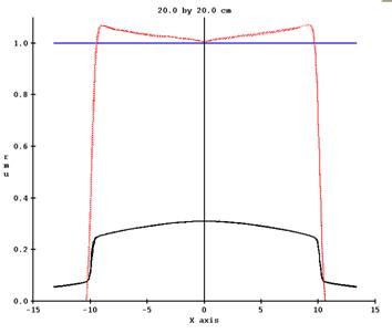
It is possible, however, that for fields that have a large dimension but are not open fields that this scheme will over compensate the profiles. The EPID kernels are fitted to give the correct dose on the central axis only.

Air Gap Correction

Additional data is needed to correct for geometry which deviates from isocenter at the center of the patient. As shown above, the dose at the EPID is insensitive to changes in the exit surface to EPID distance (air gap). However, errors are more significant for larger fields sizes. A method is provided to make corrections. By normalizing data for each field size, we are employing differences rather than absolute values. The differences are less dependent upon a particular machine, so we can use one set of data on more than one machine.

The data is to consist of images taken for a range of thickness, field size, and air gap. The same set of field sizes must be used for all thicknesses, but the air gaps can be different. The air gaps to start from the largest possible to the smallest for any field size, but need not be the same for all thicknesses and field sizes.

For each field size and thickness, a 2^nd order polynomial is fitted to the central axis signal value versus air gap. The curve will be extrapolated to zero field size and extended in the other direction. Once the minimum of the parabola is reached, the curve will just extended at that minimum. Below is an example plot for 30 cm thick, 20x20 cm field size:

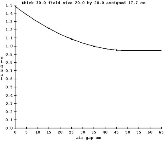
The field size must be generated by some metric that will account for the amount of scattering from the radiation field since modulated fields are not open square and rectangular fields. For each field image, the maximum intensity is found, and all other pixels are divided by that. The pixels are then all summed up, multiplied by the area of a pixel, the square root taken, and demagnified to 100 cm. In the above example, an equivalent field size of 17.7 cm was computed for the image of a 20x20 cm field (demagnified to 100 cm). While something of a loose metric, it provides a means of a common measure for all radiation fields.

For any given thickness, the curve is normalized to 1.0 for the air gap from the equation:

Air gap cm = EPID SID cm – (100.0 cm + ½ X thickness )

For 30 cm thickness and 150 cm SID, the normalization is to an air gap of 35 cm. In application, the data is renormalized to what ever SID was used for the EPID kernel data. It is therefore important that the EPID kernel images be taken so that the above equation gives the correct air gap for a given thickness. On a pixel by pixel basis, given the air gap, thickness, and field size, a correction factor is interpolated from the three dimensional air gap correction table and applied to that pixel value. The deconvolution has already accounted for the field size response of the EPID. Here we are correcting for change in intensity based on measured data due to change in air gap from the nominal measurement used to fit the exit EPID kernel.