This program is provided to measure the 50% edge of a field using an EPID or equivalent imaging system. This can be used to verify the leaf position of a multi-leaf collimator (MLC). The program can produce a report for a defined test, such as one or a series of parallel openings. Following several journal papers, we will call this a GardenFence test to distinguish from what we are calling Picket Fence below.

The program also provides analysis for Picket Fence, which we here define to be that in AAPM report 72, Task Group 50, on page 31. With Picket Fence we analyze the width of the gap detected and the center of the gap (which can be a dip or a bump in the dose) for each leaf.

Issues Involved

In using this program there are several issues to consider:

The EPID has finite resolution of the order of 0.025 to 0.078 mm pixel size.
The flood correction view adjusts all pixels to read the same number, removing the effect of the flattening filter from the image.
The EPID radiologically looks like a phantom denser than water.
Leaf edge is generally defined at the 50% fluence point (page 16, 30, AAPM Report No. 72, TG 50) relative to the value at the interception with the major X or Y axis.
The EPID is energy response sensitive, and the spectrum under a leaf is different than in the open field. For example, using an EPID to measure the wedge factor of a 60 degree wedge missed the factor by 16%.

The pixel size of the EPID will introduce an uncertainty of the order of + or – half the pixel dimension. The program does sub-pixel interpolation from center of pixel to center of pixel. Removing the effect of the flattening filter will give a different shape of the field than what is otherwise measured, as with x-ray film. The Varian Portal Vision system is usually set to multiply the off axis effect back into the data from a profile measured in water at dmax. Program MlcGapTest can otherwise multiply back in the same effect when doing a deconvolution from in air measured data. In either case, the field shape is not directly measured and this may have some effect on the end result as the 50% point may be off axis considerably depending upon the field size set. Since the EPID has internal scatter, the effect will be similar to putting an x-ray film at depth in a phantom and measuring the profile at depth instead of in air. Adding scatter to both a point on axis and a point off will change the relative difference between the points. This can effect the location of the 50% fluence point. Program MlcGapTest provides a deconvolution process, whereby the image is convolved with the inverse of the point spread function (the kernel). In effect, this is a high spatial frequency pass operation. However, the process used to develop the point spread function, the kernel, fits the kernel to optimize getting the fluence so that the correct dose in water is computed from the converted image. Edge effects are not so important nor controlled in the fitting process and this may have an effect on results when looking for a field edge to the accuracy expected for testing leaf positions. Further more, we have not seen a significant difference between using the raw image versus the deconvolved image. At present we have not provide a way to restore the in air off axis ratios separate from doing the deconvolution.

The above issues may require comparing use of this program with an EPID with the traditional method of using x-ray film. See the separate test report form provided for this purpose. However, if determining the leaf position in a narrow gap, the issues above will have less of an effect. A simple test might be to look at a 10x10 field set with the collimator jaws and see how close the program finds the edge.

Program Operation

Run program MlcGapTest. This program can be selected from DosimetryCheckTasks.under “Other Utilities”.

Select Accelerator

First select the accelerator and energy. This is a convenience provided so that the program can automatically retrieve the current deconvolution kernel. Also the energy can then be check against the image file you read in. Shown below is the toolbar to select the machine and energy:

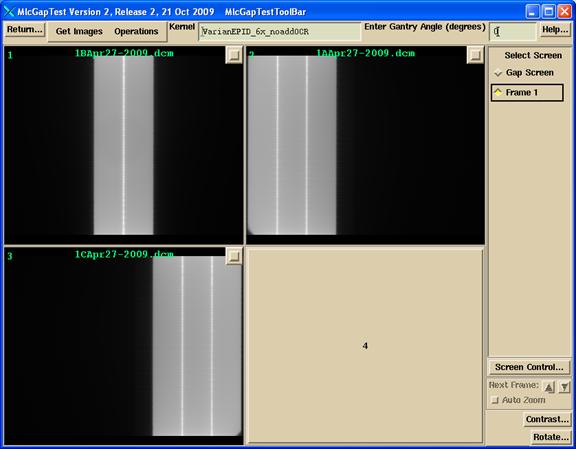
Centering images

You can choose to use one or two images made by the jaws with a narrow slit to define the x and y axes independent of the MLC. If you have only one set of jaws, you can rotate the collimator 90 degrees to get the orthogonal direction. Images are selected with file selection box popoup. The one or two jaw centering images will be displayed in frames one and two as shown below. You can choose not to read and use these images for centering and only use the MLC gap image for centering, but you would be assuming you can rely on the MLC for that function.

Note that in selecting an image, you would normally only select one image at a time. Clicking on more than one image will result in the selected images being added together for display. That would be the case if you are reading in a Varian EPID Picket Fence image that was integrated into three separate images.

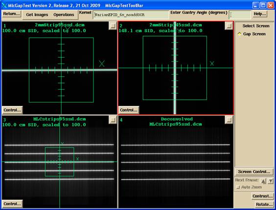
The image to be measured will be displayed in frame three, bottom left, as shown above. This deconvolved image from frame 3 will be displayed in frame four. The original pixel size of these images are retained. However, they presently must be integrated EPID images from Siemens, Varian, or Elekta.

Locate Field Tool

The locate field - centering tool will display in frames one through three simultaneously as shown, so that any of those three images can be used to define the center. The scale will be adjusted from the SID of the image to show distances at 100.0 cm.

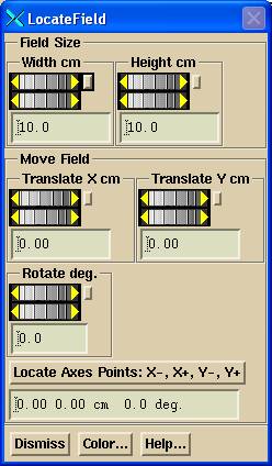The field size controls are provided to match any rectangular field you might want to match for centering. You can then translate the central axis to match any of the two jaw images or the MLC gap image. Rotation is not likely to be needed for an EPID image but is provided nonetheless.

The locate axis points will allow you to click them mouse (left button) locating in the following order: a point on the left (minus) X axis, a point on the right (plus) X axis, a point on the bottom (minus) Y axis, and a point on the top (plus) Y axis. These points do not have to be all on the same image. So in the example above, you could locate the X axis with image 1 and the Y axis with image 2. The program will then solve for the central axis location and any rotational correction. Dismiss this control when done. The found coordinate system will be applied to all four images.

Measuring Leaf Edges

You must select under the Operations pull down to deconvolve the image in frame 3, with the selected deconvolution kernel shown on the MlcGapTest ToolBar, to produce the deconolved image in frame 4. You may decide that working with the deconvolved image is not necessary.

The tool to show a profile through the image will work on any of the four

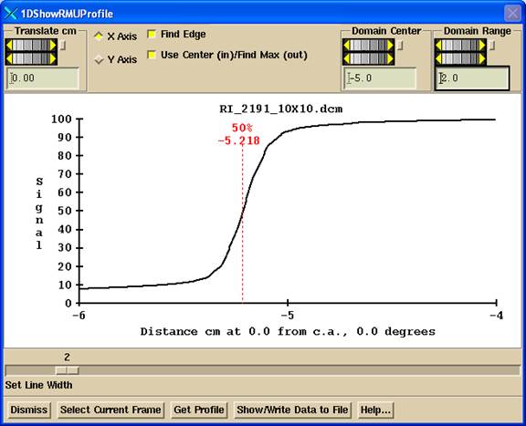
images displayed. Simply select a frame with the left mouse, the frame will be outlined in red as the current frame, and then on the below control hit “Select Current Frame”. Use the translate control to move the line now drawn on the selected frame. Use the radio buttons to select the X or Y axis. Then hit the “Get Profile” button to get and draw the profile.

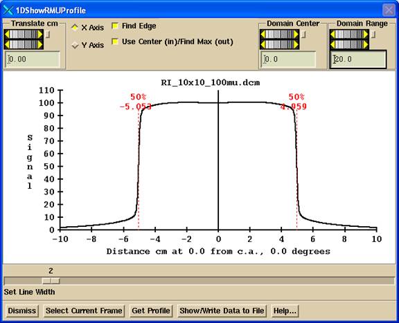
Shown above is the display for a 10x10 images formed with jaws without deconvolution (image in frame 3). The 50% edge is found on the left and right. 50% is taken of the profile where it crosses the major axis X or Y axis when the “Use Center” toggle button is in. This number may be different from the central axis value. The data is otherwise normalized to 100% of the point on the central axis. When the “Use Center” button is out, the maximum is searched for. The “Fine Edge” button turns on and off finding an edge.

Domain Plotted

You can use the Domain Center and Domain Range control so zoom in on some part of the curve.

Translate Control

Use the Translate control to move the line where the profile is to be taken. Shown below is the profile through the deconvolved image of above. Note the positioning line drawn on the image. The line will always be parallel to the X or Y axis, as defined by the centering operation, should there be any rotation of the beam’s eye view coordinate system.

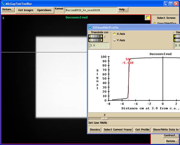
You can also select the Y axis instead of the X axis with the radio box provided..

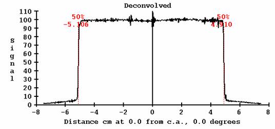
Deconvolution

Be aware that the deconvolution process is a high pass operation and some times will amplify noise as shown below. Compare to the above image from a different 10x10 image. This effect is less in DosimetryCheck because the deconvolved images are first reduced in resolution to a pixel size of 1 mm, which is a smoothing operation.

MuliLeafGeometry File

In order to use the below Garden Fence or Picket Fence tools, there must be a file that defines the multi-leaf collimator for the chosen machine. This file with name MultiLeafGeometry goes into the top directory of the particular machine. The file follows our text file standard where /* to */ is a comment that the program does not read, and // to the end of a line is also a comment. Text that is to be read is set of with <* to *>. Numbers are set off with white space. An example file for a Varian machine follows below. Note change to version 3 file format from version 2, where a parameter was added to specify the order for labeling the leaf pairs. If +1 the order is minus coordinate to positive coordinate. In the example below, -19.70 is leaf pair one. If -1 the labeling is reversed and -19.70 is leaf pair 60.

/* file format version: */ 3

/* file type: 12 = Multi-Leaf geometry */ 12

/* transmission of leaf is under each energy directory */

/* direction for labeling of the leafs in MlcGapTest program:

+ 1 is minus coordinate to positive.

- 1 reverses the order. */ -1 //this parameter added in version 3

// file format.

/* NOTE: program is limited to ONLY X or Y leaves, but not both.*/

/* X leaves flag: 0 none, 1 leaves */ 1

/* see Y leaves below if flag is 0 */

// information follows only if flag is 1

/* source distance to bottom of leaf (cm) */ 53.8

/* Maximum opening width */ 40.0

/* Minimum opening width */ 0.0

/* number of leaf pairs: */ 60

/* leaf center coordinate (cm) followed by leaf width,

followed by limits of the minus left, then limits of

the positive leaf: */

-19.70 1.4 -20.1 20.1 -20.1 20.1

-18.50 1.0 -20.1 20.1 -20.1 20.1

-17.50 1.0 -20.1 20.1 -20.1 20.1

-16.50 1.0 -20.1 20.1 -20.1 20.1

-15.50 1.0 -20.1 20.1 -20.1 20.1

-14.50 1.0 -20.1 20.1 -20.1 20.1

-13.50 1.0 -20.1 20.1 -20.1 20.1

-12.50 1.0 -20.1 20.1 -20.1 20.1

-11.50 1.0 -20.1 20.1 -20.1 20.1

-10.50 1.0 -20.1 20.1 -20.1 20.1

-9.75 0.5 -20.1 20.1 -20.1 20.1

-9.25 0.5 -20.1 20.1 -20.1 20.1

-8.75 0.5 -20.1 20.1 -20.1 20.1

-8.25 0.5 -20.1 20.1 -20.1 20.1

-7.75 0.5 -20.1 20.1 -20.1 20.1

-7.25 0.5 -20.1 20.1 -20.1 20.1

-6.75 0.5 -20.1 20.1 -20.1 20.1

-6.25 0.5 -20.1 20.1 -20.1 20.1

-5.75 0.5 -20.1 20.1 -20.1 20.1

-5.25 0.5 -20.1 20.1 -20.1 20.1

-4.75 0.5 -20.1 20.1 -20.1 20.1

-4.25 0.5 -20.1 20.1 -20.1 20.1

-3.75 0.5 -20.1 20.1 -20.1 20.1

-3.25 0.5 -20.1 20.1 -20.1 20.1

-2.75 0.5 -20.1 20.1 -20.1 20.1

-2.25 0.5 -20.1 20.1 -20.1 20.1

-1.75 0.5 -20.1 20.1 -20.1 20.1

-1.25 0.5 -20.1 20.1 -20.1 20.1

-0.75 0.5 -20.1 20.1 -20.1 20.1

-0.25 0.5 -20.1 20.1 -20.1 20.1

0.25 0.5 -20.1 20.1 -20.1 20.1

0.75 0.5 -20.1 20.1 -20.1 20.1

1.25 0.5 -20.1 20.1 -20.1 20.1

1.75 0.5 -20.1 20.1 -20.1 20.1

2.25 0.5 -20.1 20.1 -20.1 20.1

2.75 0.5 -20.1 20.1 -20.1 20.1

3.25 0.5 -20.1 20.1 -20.1 20.1

3.75 0.5 -20.1 20.1 -20.1 20.1

4.25 0.5 -20.1 20.1 -20.1 20.1

4.75 0.5 -20.1 20.1 -20.1 20.1

5.25 0.5 -20.1 20.1 -20.1 20.1

5.75 0.5 -20.1 20.1 -20.1 20.1

6.25 0.5 -20.1 20.1 -20.1 20.1

6.75 0.5 -20.1 20.1 -20.1 20.1

7.25 0.5 -20.1 20.1 -20.1 20.1

7.75 0.5 -20.1 20.1 -20.1 20.1

8.25 0.5 -20.1 20.1 -20.1 20.1

8.75 0.5 -20.1 20.1 -20.1 20.1

9.25 0.5 -20.1 20.1 -20.1 20.1

9.75 0.5 -20.1 20.1 -20.1 20.1

10.50 1.0 -20.1 20.1 -20.1 20.1

11.50 1.0 -20.1 20.1 -20.1 20.1

12.50 1.0 -20.1 20.1 -20.1 20.1

13.50 1.0 -20.1 20.1 -20.1 20.1

14.50 1.0 -20.1 20.1 -20.1 20.1

15.50 1.0 -20.1 20.1 -20.1 20.1

16.50 1.0 -20.1 20.1 -20.1 20.1

17.50 1.0 -20.1 20.1 -20.1 20.1

18.50 1.0 -20.1 20.1 -20.1 20.1

19.70 1.4 -20.1 20.1 -20.1 20.1

/* Y leaves flag: 0 none, 1 leaves */ 0

Gantry Angle

If you enter a gantry angle in the text field provided on the MlcGapTextToolBar, the angle will be reported on the test reports below for Garden Fence and Pickett Fence. The angle will be read from the image selected for frame 3. If you wipe the text field clear, the angle will not appear on the reports.

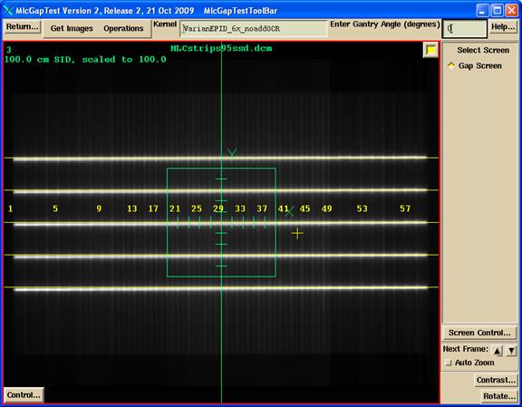
Garden Fence

We define Garden Fence as a series of one or more rectangular fields that are separated. In the example show below the field opening is 0.5 cm wide, the full width of the MLC, with opening centered at -6 cm, -3 cm, 0 cm, +3 cm, and +6 cm (defined at the distance of 100 cm SSD). See the example image below. A wider gap might be more desirable than the example shown below. The reason being that a wider separation will leave less tail from one leaf adding to the profile for the opposed leaf. On the other hand, issues discussed above concerning the EPID might become a greater contributing factor.

Garden Fence Test File

To define the test, you must create a text file that specifies the test you are going to do. Below is the test file for the example shown here. The file goes into your data directory (defined by the file DataDir.loc in your program resources directory, which is in turned defined by the file rlresources.dir.loc, see the System2100 manual) under a sub-directory called “MLCGFence.d”. An example file is:

/* file format version */ 1

// file to specify a Garden Fence MLC leaf gap position test.

/* tolerance in cm */ 0.1

// all coordinates are at 100.0 cm SID in cm

/* number of gaps: */ 5

// for each gap specify center coordinate and width

/* gap coordinate: cm gap width cm */

-6.0 0.5

-3.0 0.5

0.0 0.5

3.0 0.5

6.0 0.5

See also the System2100 manual for our text file format specification. Basically, anything from /* to */ is NOT read by the program, or anything from // to the end of a line. These are comments for user information only and are used to define what the file entries are.

The file with the data:

1 0.1 5 -6.0 0.5 -3 0.5 0.0 0.5 3.0 0.5 6 0.5

for example is read exactly the same.

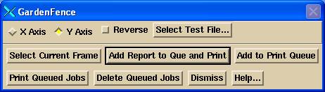
Garden Fence Popup Tool

Under the “Operations” pull down select Garden Fence. You will get the below pop up. Hit the “Select Test File” button and select your test file. Then select either the lower left image or lower right image (if you are going to use the deconvoluted version of the image) to make that frame current, and hit the “Select Current Frame” button. You must select a test file, then select the image you want to analyze, then hit the “Select Current Frame”. The current frame is outlined in a red border. Note the button on the upper right hand corner of all images. Selecting that will make that frame occupy the entire screen.

Example Garden Fence Gap Image

An example Garden Fence image is shown below. [Under the “Get Images” pull down select “Read MLC Gap Image” before you can do the step above.] The program will draw a yellow line where it expects the center of your gaps are from the test file you selected. Select the “Y Axis” toggle buttons if your image is rotated 90 degrees. Likewise hit the “Reverse” button to rotate the test pattern 180 degrees to align your test with the image. The program counts from the most negative leaf in BEV coordinates as leaf pair 1 for order direction 1 in the multi leaf geometry file, otherwise counts the leafs in the opposite direction. Every fourth leaf is labeled here.

You might want to put print this image (see Printing in the System2100 manual). Click on the image and hit the P key for the frame or the S key for the entire screen, and add to print que. Then to generate and print your report hit the “Add Report to Que and Print” button. You also have the option of adding to the print que and printing later after adding other screen captures or reports.

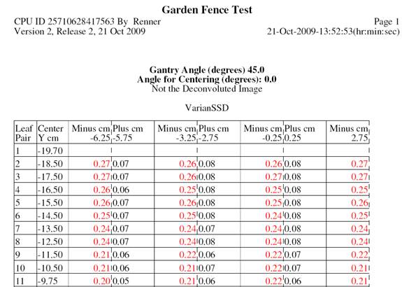
Garden Fence Report

The report will label in red any leaf position that is outside of tolerance (specified in your above test file that you selected). The leaf position is found by finding the maximum signal in the gap between a leaf pair, and then finding the position of ½ of the signal to define the leaf edge. The top row of the report shows were the leaf edge is expected for each gap. Each successive row shows the pair number, the center coordinate value of the leaf pair in BEV coordinates, and the error measured for the leaf edge, all in cm. Positive means the leaf was more positive than expected in BEV coordinates, negative more in the negative direction.

An excerpt from the report is shown below.

Picket Fence

The Picket Fence test is defined in AAPM Report No. 72, Task Group No. 50, page 31.

The name of this test is not assigned as “Picket Fence” in that report. We are using that name to distinguish from Garden Fence above, and choosing these names because of references we found in two papers published in Medical Physics that used this terminology.

A rectangular area is exposed, and then the rectangular area is moved so that one side abuts the prior area. If leafs were precisely at the 50% transmission edge and the tails matched the shoulders exactly, the abutting edge would not be detectable. Otherwise there may be a dip or a bump in dose. Shown below are two examples:

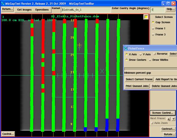
Example Elekta Picket Fence Image

An example Elekta Picket image is shown below:

A profile through the pattern is shown next:

Note that there is a dip between the exposed areas. Further, that there is no 50% of the maximum area. Therefore we cannot compute a leaf edge position. We can compute a gap width defined as the edge one half way between the maximum and minimum.

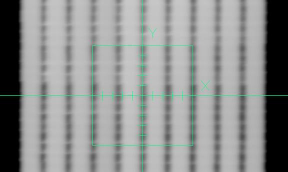
Example Varian Picket Fence Image

Below is the image of Varian Picket Fence. Here three images were selected and added together.

The sum of the three images:

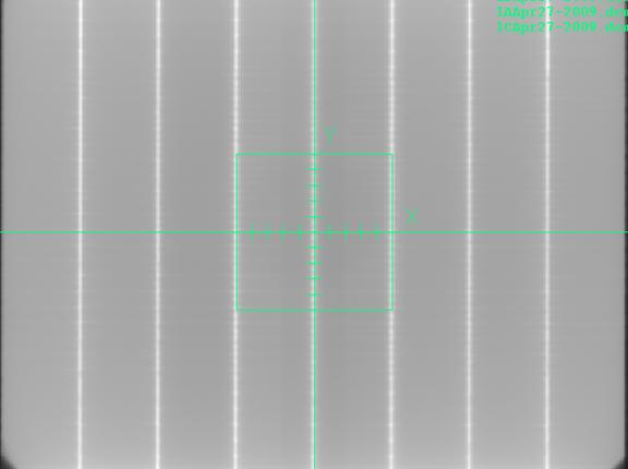
And below is a profile through the image:

Here we have a bump. Again as in the case above, we do not have 50% of the maximum and cannot compute leaf edges. Rather we compute the bump or dip width and center using the location along the curve that is ½ between the maximum and minimum.

Picket Fence Test File

We define our test similar to the garden test file above. The file goes into data.d\MLCPFence.d. An example file for the above Elekta case is shown below.

The pickets must be in order by the coordinate.

/* file format version */ 1

// file to specify a Picket Fence MLC leaf gap position test.

/* center tolerance in cm */ 0.1

/* width tolerance in cm */ 0.05

// all coordinates are at 100.0 cm SID in cm

/* number of pickets: */ 9

// for each picket specify center coordinate and width

/* picket center coordinate: cm picket width cm */

-10.0 0.65

-7.5 0.65

-5.0 0.65

-2.5 0.65

0.0 0.65

2.5 0.65

5.0 0.65

7.5 0.65

10.0 0.65

Notice that the only difference is here we have a separate tolerance for center and width. The tolerance, center, and width to enter into the file are to be determined by the user.

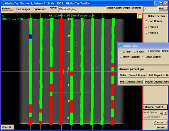
Picket Fence Popup Tool

Shown below is the Picket Fence popup tool:

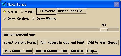
An additional issue is the minimum difference between the maximum value along a profile and the minimum value at which a dip or bump will be assumed to have occurred. The default is the minimum value must be <= 90% of the maximum value. If not, the leaf pair is ignored and not reported on.

You must select a test file, and then select the image you want to analyze. Then hit the “Select Current Frame”. The current frame is outlined in a red border. Note the button on the upper right hand corner of all images. Selecting that will make that frame occupy the entire screen

Picket Fence Report

The program will compute the width and center of each dip or bump, and compare to the expected values from the test file. Across the top of the report is the expected center coordinate and width in cm. For each leaf pair the center coordinate and width is shown. The leaf pairs are labeled according to the direction specified in the multi leaf geometry file (i.e. is the most negative coordinated the first leaf pair or the last).

An excerpt from the test report is shown below:

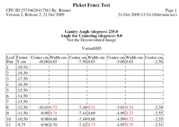
A width too large is shown in red. Too small in blue:

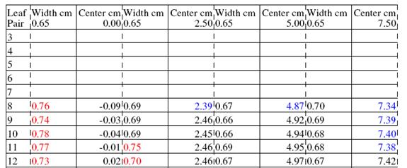
Likewise a center value too negative is in blue, too positive in red.

Picket Fence Color Display

A color display of the results can be shown on top of the picket fence image for a visual reference.

Picket Fence Color Width Display

Shown below are the widths. If the width is within tolerance, the width is green. Too large a width is in red. Too small a width, than blue.

Picket Fence Color Center Display

Next is the same display of the widths, but here the coloring depends upon the center value. Within tolerance is green, too negative is blue, too positive is red.