Program ConvertEPIDImages has been provided to read in images from the Varian, Siemens, and Elekta portal imaging systems and to convert them to fluence files for input to Dosimetry Check. For Elekta systems you must first run the IviewToDicom utility to convert to Dicom files. This program will read Varian files and files written by IviewToDicom directly. For Siemens, run the Convert Siemens version of this program. For the Map Check, PTW 2D, and Matrixx arrays, use the ConvertMapCheckImages, ConvertPTW2DImages, and ConvertMatraixxImages executable versions of this program.

Calibration, Deconvolution, In Air Off Axis Ratio

Images must be calibrated in a fluence unit, here defined to be the relative monitor unit (rmu), which is the intensity relative to the intensity on the central ray of a calibration field size, typically 10x10 cm.

The effect of scatter within the detector itself must be removed to convert the image back to a fluence image. A two dimensional deconvolution with the inverse of the point spread function is done to accomplish this.

The flood view correction for an EPID corrects for the different response of the EPID to the change in the x-ray spectrum off axis and so also removes the off axis variation inherent in radiation fields due to things like the flattening filter. If removed, it must be restored. See the note below on shifting the EPID or detector.

There are three options for the steps above:

Option 1:

This conversion consists of four steps:

Convert the pixel values to relative monitor units (RMU) by which every pixel is mapped to the monitor units that would produce the same pixel value at the center of a 10x10 cm field size.
Deconvolute the image with a kernel that removes the effects of the imaging device, restoring the image to fluence.
Multiply the image by the measured in air off axis ratio to restore the in air shape of radiation fields. (Deviation from a flat distribution is mainly caused by the flattening filter.)

Option 2:

Varian will multiple in off axis ratio data measured at dmax in water. The dmax curve is nearly the same as an in air curve. Therefore, one may use the field image as is and not multiple in the in air curve. Further, the user has the option of supplying their own data. Only steps 1 and 2 above would be performed. This would be the option to use for other devices that are not corrected by a flood view.

Option 3:

For the case where in water OCR has been multiplied in, first remove the in water off axis ratio data (at dmax) that the image was multiplied by. This should restore the integrated image to after correction by the flood view. Then after deconvolution, multiply in the in air data. This works slightly better but there is hardly any difference.

The method is set at the time the kernel is fitted (see below) and is passed in the kernel parameter file. The same kernel can be used for either option and the method could be switched by editing the kernel file.

These steps require data. The first step requires a calibration curve that can be generated from one or more images of a 10x10 cm field at different monitor units. This curve may have to be regenerated depending upon the stability of the imaging system. Note: if you calibrate your treatment machine to a different field size, use that field size. For integrating systems, one single calibration field (10x10 cm) should suffice based on the assumption that the response is linear and has a zero intercept.

The second step requires a deconvolution kernel, and the third in air off axis ratio data.

The third option requires the same in water off axis data that was used by the Varian EPID software.

The kernel generation for deconvolution is covered in a separate document: “Fitting Deconvolution Kernels for Electronic Portal Imaging Devices (EPID).” A link to the kernel fitting toolbar is provided in this program as shown below.

The in air off axis ratio curve that is part of the accelerator data base for a particular energy is used directly. This requires that the accelerator and energy be selected at the time of conversion. This curve is a circularly symmetric curve as a function of radius (equivalently as a function of angle with the central ray). It is measured with a detector in air but with a build up cap. We recommend you use something like brass instead of plastic. Generally you would scan the diagonals of a 40x40 field at any convenient distance, and take an average of each of the four legs.

The image files are written out in “Field Dose” format in rmu units for direct input by Dosimetry Check (see the Dosimetry Check manual). In Dosimetry Check for each treatment portal (beam) the user must select the corresponding Field Dose fluence file. Dosimetry Check will automatically select the files, adding them together if necessary, if the files are sorted into the proper beam folders as described below. The resultant field fluence is then stored separately under the beam name (in the beam’s directory under the plan in the patient’s directory).

The image files may here be converted as a group.

Shifting the EPID or Detector

If the EPID or detector is calibrated with flood field, then fields should be integrated with the EPID or detector at the same location and distance for the OCR to be properly restored. Alternately, a flood view correction can be applied in the conversion process as described below.

When the flood correction is done in the calibration of the EPID, the individual pixel gains are adjusted to give the same value for the entire image. However, the flood field is not flat, and so this calibration wipes out the "in air off center ratio effect (OCR) due to the effect of the flattening filter and other variations of intensity off axis. Hence that curve has to be restored and it is perfectly appropriated to simply multiply it back it since this is a fixed fluence function.

What happens, however, if you move your EPID off axis, say for argument 5.0 cm? Let us look at some in air OCR data (measured on a Varian at 6x):

Tangent OCR where Tangent x 100 cm = distance cm from central axis at 100 cm

0.0000   1.0000
0.0050   1.0008
0.0100   1.0034
0.0150   1.0059
0.0200   1.0084
0.0250   1.0102
0.0300   1.0110
0.0350   1.0131
0.0400   1.0172
0.0450   1.0210
0.0500   1.0243
0.0550   1.0263
0.0600   1.0273
0.0650   1.0282
0.0700   1.0289
0.0750   1.0297
0.0800   1.0305
0.0850   1.0310
0.0900   1.0311
0.0950   1.0316
0.1000   1.0324
0.1050   1.0332
0.1100   1.0342
0.1150   1.0347
0.1200   1.0348
0.1250   1.0350
0.1300   1.0355
0.1350   1.0362
0.1400   1.0373
0.1450   1.0382
0.1500   1.0391
etc…

So let us assume that the gain of all the pixels are all the same (and we are assuming circular symmetry). Further, we will here assume that the in air OCR is multiplied in relative to the central axis, not where the central axis was when the flood view correction was done.

Pixel values for a flood view at 5 cm will be 1.0243 and at 10 cm will be 1.0324. So after the flood view correction a point 5 cm from the c.a. will be multiplied by 1/1.0243 and at 10.0 by 1/1.0324

Upon restoration of the curve, we once again have values of 1.0243 at 5 cm and 1.0324 at 10 cm. I.e., using pixel value = signal times flood view correction times in air OCR:

at 0:    pixel value = 1.0 x 1/1.0 x 1.0 = 1.0
at 5:    pixel value = 1.0243 x 1/1.0243 x 1.0243 = 1.0243
at 10: pixel value = 1.0324 x   1/1.0324 x 1.0324 = 1.0324

Suppose now however that the EPID is shifted 5 cm with the center of the EPID now at 5 cm in the above OCR table. Because we take the 10x10cm calibration field with the EPID at the same position we will get the correct rmu on the central axis of the radiation field. However, consider what happens to the values at + and - 5 cm closer and further from the machine along the direction of the shift:

Using again:

pixel value = signal times flood view correction times in air OCR

at 0: (prior center of EPID) pixel value = 1.0243 x 1/1.0000 x 1.0243 = 1.0492

at 5: (central axis)       pixel value = 1.0000 x 1/1.0243 x 1.0000 = 0.9763

at 10:                                     pixel value = 1.0243 x 1/1.0324 x 1.0243 = 1.0163

Normalizing to the central axis (since we calibrate the field there) we will have the final result:

0 cm           5 cm             10 cm
1.075       1.000             1.041

But correct values are:
1.0243     1.000             1.0243

At present, this program will restore the in air OCR relative to the position of the central axis and not the center of the imaging device. This is applicable if you do your own flood correction here as described below.

This may be incorrect as shown immediately above. The Varian system will multiply in an OCR curve, in which case program ConvertEPIDImages should not also restore the OCR. Whether Varian takes into account any shift from the flood view position is not presently known to this author. The Varian system also allows for a shift in source image distance (SID). A change in SID results in a change in magnification of the OCR curve. Reapplying the OCR for a different magnification will also result in some distortion, although perhaps not as large an effect as a shift if the OCR has a nearly constant slope off axis. Hence the present recommendation that if flood view corrected, perform the flood view at the same center and SID that the EPID will be used acquiring data for Dosimetry Check.

For the rare case when the EPID must be off axis, you can read in a flood view at the time and process it as described below.

Choose Accelerator

The use must first select the accelerator and energy for which the images were obtained. The choose accelerator and energy toolbar is shown below:

Simply pick the accelerator from the pull down list and then the energy, and then hit the “Continue…” button.

EPID Toolbar

The EPID toolbar is shown below:

The options pull down is shown:

We will cover each option below.

Patient

The patient must first be selected or a patient entry created. The other buttons on the pull down will be grayed out until a patient entry is defined. Resulting fluence files are written to the patient directory under the patient’s name in sub-directory FluenceFiles.d. The treatment plan and stacked image set should be stored under the same patient entry.

A patient entry is actually a directory name made out of the patient’s name in the patient directory. The patient directory is defined by the file PatientDirectory.loc in the program resources directory (which is in turn defined by the file rlresources.dir.loc in the current directory).

Sort Image Files

An option is provided to sort the images files in a directory (folder) for the case when it is not obvious which image files belong to a particular patient, plan, energy, or field. You will get a file selection dialogue popup as shown below:

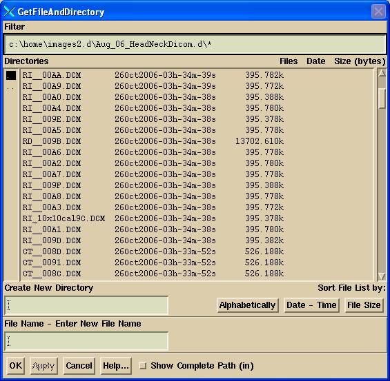
Navigate either by typing in a path in the filter (be sure to end with / or \ and *) or use the left column to select directories up or down. You are not restricted in your navigation. When you see the images files on the right column, hit the OK button.

Non Dicom image files will be ignored. The Dicom image files will be MOVED to subdirectories of the directory you have selected. The subdirectories will go in the order:

Patient Name

Date (of the image)

Study Description with the energy appended (such as 6x)

Image Label (only if more than two images)

If a study description or image label already exist, a new one is created with _n appended to the prior name, where n will be a counter (note this can only happen if the same image date). Note also that different energies are separated into different folders.

The text used for the above is that found in the header of the respective Dicom image files. All IMRT files are to be copied to the same directory under the Study Description, but since there is no way to tell the difference between an IMRT image file and an IMAT image file from the header information, if there are more than two images with the same patient name, date, and study description, it is assumed that they are IMAT images and are put in a directory under the image label name. Since an MLC carriage shift for an IMRT beam can result in two separate images, 2 or less image files are not put under a separate image label directory. The file name will be changed to the image label name with the Dicom time field appended and a number 1 or 2 appended if there are two such image files.

You will get a popup reporting of the number of image files found for each patient, date, study description, and image label.

Image files may be then selected as described below for conversion by navigating down the directories created above to the desired images, and then “Select All” or selected the images to be converted.

Copy Partial Plan

Use this option to copy an exiting plan, giving it a new name. Prior fluence files and computed dose will not be copied. Use this option if you want to look at dose reconstruction for a plan that you have already done and do not want to lose the prior dose reconstruction. The program will suggest appending the current date to the name of the plan you are copying from for copied plan name.

Convert Images

Use this option to convert images once a calibration curve and kernel is available. You will first get a file selection box to select the EPID files to be converted:

Select Input Files

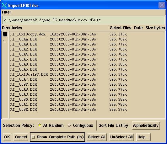
Select all the fields for the same machine and energy for the case. Then hit the OK button.

The “At Random” toggle button will let you select particular files. The “Contiguous” toggle button will let you select a range of image files. Select one file, then hold down the shift key while you select a file that brackets the files you want to select.

The default directory where the files selection box will start at is defined in the file NewEPIDImagesDirectory.loc in the program resources directory. This file can be edited to move that location. Files with the letters “cal” (case insensitive) in them are assumed to be calibration files rather than files of images to be converted. If only one such calibration file it will be assumed to be used for all files. If more than one and if the files to be converted are for different gantry angles, then the calibration files will be initially assigned to files with the same gantry angle. The user may change the assignments. File CalFileDirectory.loc in the program resources directory contains the default path where the file selection box will start to select a calibration file.

Convert to Fluence Files

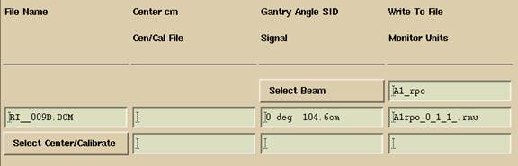
The selected files will then appear in the next popup:

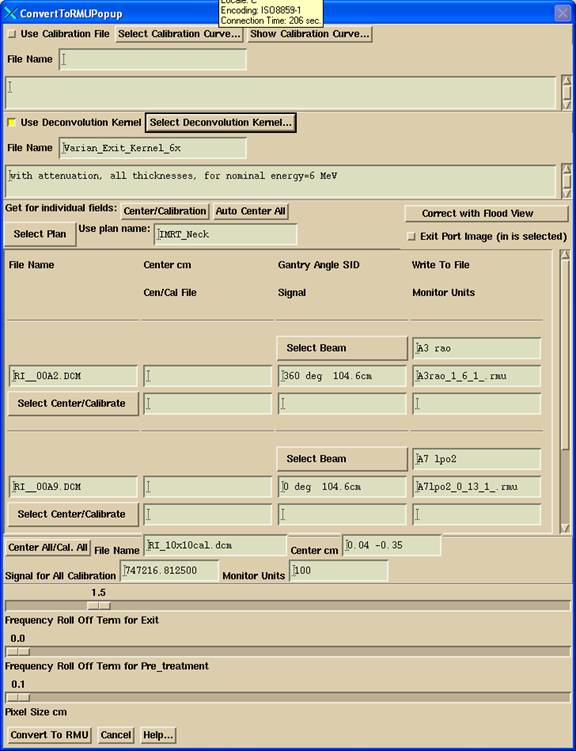
There are two primary issues to be dealt with here, calibration and centering. Because the imaging device may be subject to sagging as the gantry rotates for some mounting systems, a provision is made here to allow each image to be centered and calibrated separately. Calibration would require a 10x10 cm field (assuming that is the calibration condition for the machine) with a known monitor unit exposure. This same field can be used to define where the central ray is at a particular gantry angle. You would not normally use the IMRT integrated image for centering because the field boundaries are not well defined relative to the central axis.

For each selected file to be converted, there are three rows with text fields and the Select Center/Calibration pull down menu. The file to be converted is shown in the first column second row text field. The current center coordinates are shown in the second column second row (blank is 0,0). The gantry angle, if known, and the source image distance (SID) is shown in the next text field. In the last column second row is the file name that will be used for the resultant rmu file that will be written into the particular patient’s directory (see Plan name and Beam name below). The output file holds the fluence image for the measured field. The user may change this file name. All the files that are to be written to the same folder must have unique names.

Calibration and Centering

You can calibrate and find the central ray for each field file individually. If calibration files were not included in the original selected list, hit the “Center/Calibration” to select more files. The first text field on the third row displays the Center/Calibration file name, if one was selected, the next text field shows the signal value from the center-calibration image, and the last text field is where the monitor units are to be entered if images are to be individually calibrated. Enter a monitor unit value here followed by the enter key will enter that monitor unit in all the mu text fields that are below the one entered. If this is not desired, don’t hit the enter key after entering the number. The monitor units will also default to the value last used for the machine and energy selected.

Shown below is an example of individual calibration, where a calibration file has been selected for an individual file. The pull down menu may be used to select a different calibration file, or the association removed by selecting “No Selection”, or the text fields erased by selecting Reset.

Center all, Calibrate All

If you are not going to enter a separate calibration field for every image, you can select a file to use for all the fields by hitting the “Center All/Cal. All” button near the bottom of the popup. You may use the same image to center all images (see below) and to specify the calibration. At the bottom of the popup is a text field where the signal from the center of the centering field is shown, and next to it is where the monitor units for this field is entered. A calibration constant will be generated as the ratio of mu/signal and applied to all fields for which an individual calibration was not established. The below selected calibration curve will be ignored. If an entry is not made here, then the below calibration curve will be used (if selected) for all fields not individually calibrated.

AutoRunDC

The program will default to using the last calibration image processed for the EPID by program AutoRunDC or CalibrateEPID so that you need not enter a specific image here for this purpose. Be aware that AutoRunDC will update to use the mu you enter here and the EPID kernel that you select here. But AutoRunDC will not use the calibration image that you select here but will continue to use the last one it (or CalibrateEPID) processed.

Calibration Curve

You can generate a calibration curve. However, this is generally not needed since integration results in a linear response with a zero intercept and so can be done as above with a single point. Either hit the “Select Calibration Curve” button to select a calibration curve or create one here. Once a calibration curve is selected and used, the same curve will be the default entry here for this machine and energy. Calibration curves are stored in the data sub-directory CalDCur.d. The data directory is located by the file DataDir.loc in the program resources directory rl.dir specified by file rlresources.dir.loc in the current directory.

An entry will also be made in the data directory for each treatment machine to store the name of the last calibration file used here. A folder is made for the machine name, then the energy (such as X06), and then stored in the file EPIDcalFile is the name of the calibration file last used.

Centering Tool

You can use one file to find the central ray for all images by hitting the “Center All/Cal. All” button and selecting a calibration image file. Or you can select a calibration file for an individual file using the “Select Center/Calibration” pull down menu for each image entry. In both cases you will get a display of the calibration image. Hitting the “Control” button in the lower left hand corner of the image will bring up the centering control as shown below:

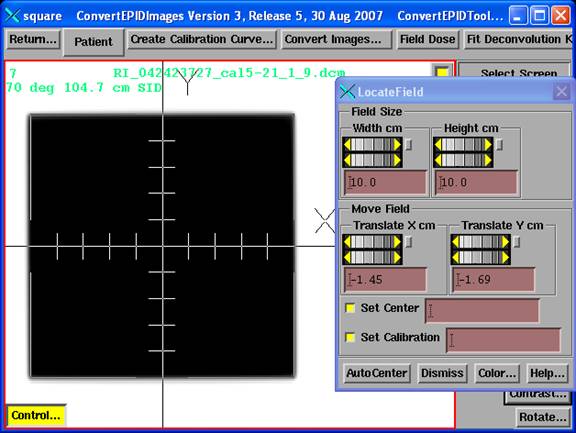
Set the field size if different from 10x10, and then use the translate X and Y controls to move the field drawing to coincide with the field image. Or try the AutoCenter button. The center off set will be shown in the above convert to dose control. Your task here is define where the central ray is relative to the treatment radiation fields. But you must also find the center signal value at the center of the calibration field. Normally this is done in one operation as shown here.

Note also the toggle buttons for Set Center and Set Calibration, each with a text field. Both buttons are normally ON (in) and the centering and center value will be forwarded to the convert to dose tool. However, you could turn one of them off to specify centering separately from finding the center signal value. This may be of use if the EPID is moved off center so that the center of a centered 10x10 would miss the EPID or be near the edge. Move the field image to define the true location of the central ray. Then turn off Set Center and move to define the center of the 10x10 calibration field to get the signal value. What is turned off will not update to the right. However, if you have two images to use, then use the one in the same location as the image to be converted to find the central ray and a second with a centered calibation image to get the center signal value.

If you used the individual method, you must then type in the monitor units used for the 10x10 cm field for the calibration to be used. The calibration factor (of monitor unit/signal) will be used as a factor to convert the pixels of the integrated selected field to RMU, with the signal value coming from the center of the calibration field. Note that it is assumed here that zero signal is zero monitor units. If you do not enter the monitor units in the text field provided, the calibration cannot be used since the numerator is not specified.

The order is to use the individual calibration if defined. If not entered, then to use the global all calibration. If that was not entered, then to use the above selected calibration curve file if one was entered. If no calibration is defined, there will be an error message.

Auto-Centering

The calibration image files are auto centered if included with the original list of files. There is a button to command auto-centering all of the calibration images that were select for individual use. For the All option, use the Control button on the image of the field.

Centering and SID correction for gantry angle

For program versions 28 Sept 2012 and later:

Corrections can be made from a table for shifts of the EPID as a function of gantry angle. This correction will only be supplied for an EPID. If using some other device (one of the other conversion utilities), this correction is not made. A file name EPIDShift.txt is to go into the specific the machine directory (not in any energy sub-folder such as X06, as the data has nothing to do with the energy of the beam). Measure the shift in x and y for gantry angles 0 to 360. An example of a file is shown below. The EPID.log file could assist you, but an entry is only made to that file when images are converted. But you can use the above centering tool for images taken at different gantry angles and record the x and y shift. The SID shift can be computed from the signal values by solving the below equation for the shift s in SID:

Signal at 0 degrees (SID + s)

------------------------- = ---------- squared

Signal at angle (SID)

where s is the shift for the EPID at the angle and SID is the distance the EPID was at for the measurements. Note, however, the table does not need to be normalized a 0 angle.

NOTE: the gantry angles are for IEC coordinates (positive is clockwise looking into the machine from the couch side, 0 degrees is beam pointed at the floor). You will have to convert your gantry angles for this table if your machine is not IEC (internally Dosimetry Check is IEC).

Given the gantry angle for the calibration field, the shift is interpolated from the below table, call the result cal_shift (for x, y, or SID). Then the shift is interpolated for the gantry angle that the image was measured at, img_shift. The difference: img_shift – cal_shift, is added to the shift from the calibration image and applied to the image for the location of isocenter and the SID of the image.

If there is a difference between clock-wise and counter-clockwise rotation, average the difference for your table. Nor are corrections made here if the shift is SID dependent.

Example file EPIDShift.txt:

/* file format version */ 1

// EPID shift in x, y, and SID versus gantry angle.

/* number of rows of data */ 13

// gantry angle here is in IEC coordinates, clockwise is positive

// rotation. Shift is where isocenter moves to relative to a fixed

// point on the EPID. Data does not have to be normalized at 0 gantry

// angle. Angle must be 0 to 360.

// Gantry Angle X shift cm Y shift cm SID shift cm

0 0 0 0

30 -0.07 -0.08 0.00

60 -0.15 -0.16 0.00

90 -0.15 -0.31 -0.51

120 0 -0.55 -1.03

150 0.08 -0.63 -1.41

180 0.24 -0.7 -1.63

210 0.47 -0.63 -1.43

240 0.47 -0.55 -1.26

270 0.47 -0.31 -0.83

300 0.4 -0.16 -0.34

330 0.24 0 -0.16

360 0 0 0.00

Deconvolution Kernel

Hit the “Select Deconvolution Kernel” to select the kernel to use. Again thereafter the program will default to the selection for the same machine and energy. An entry will be made in the data directory for each treatment machine and energy to store the name of the last kernel file used, in the file EPIDkernelFile.

Do not deconvolute images that are to be used to fit the kernel.

Unselect the toggle button if the files are to be used for fitting the kernel. The kernel fitting routine won’t accept files that have already been put through a deconvolution process. Unselecting also means that the in air off center ratio function will not be multiplied in.

Frequency Roll Off Term

This term adds a low pass filter to the image processing to attenuate high frequencies. This is generally needed for processing exit images. The deconvolution process is a high pass filter. Adding a final roll off will eliminate some spikes that high passing might introduce at sharp sudden edges. The default value of 1.5 was selected by means of trial and error. Setting this to zero will eliminate the roll off. The equation used is

e^{(-roll_off_value X spatial frequency in cycles/cm
squared)}.

The default value can be set by the file DeconvRollOff in the program resources directory (named and located by the file rlresources.dir.loc in the current directory). The file format for program versions prior to Oct 1, 2013 is:

/* file format version */ 1

/* roll off constant for deconvolution in

Dosimetry Check. Gauss term:

exp(-a q squared )

where q is spatial frequency in cycles/cm

value of a to use: */

1.5

For versions of the program on and after Oct 1, 2013, the exit and pre-treatment roll off values may be set separately:

/* file format version */ 2

/* roll off constant for deconvolution in Dosimetry Check

Gauss term: exp(-a q squared )

where q is spatial frequency in cycles/cm

default value of a for exit: */

1.5

// default value of a for pre-treatment

0.0

Pixel Size

We suggest leaving the pixel size at 1 mm for the resultant fluence file for normal operation.

Flood View Correction

It may be that you have had to shift the EPID off axis for a field. In that case, you must shoot the 10x10 at the same location, and in addition you can shoot a large flood view with the EPID at the same location. You should only process images that were taken with the EPID at the off set location. The program will then first correct the incoming image with the flood view that you read in. In this case, however:

The in air OCR is then always restored from the beam data that Dosimetry Check has irregardless of the specification in the deconvolution file.

This may be different if you normally get the OCR with the EPID image as may be the case with a Varian system.

Lastly, be aware that the edge of the image might have a large gain. The converted images might show up black in the center because of the resulting large signals at the edges. In this case restrict the area to exclude those areas.

Plan name and Beam name

You should normally down load the plan before running the program. Then select the plan that the images are for. But you can also type in a plan name and a beam name instead if you have not done so, or if you want to store the converted files under some other folder. And if a plan name is not entered, the output files will not be in a subfolder starting with a plan name. If you also do not enter a beam name, the files will be just in a subfolder IMRT (or IMAT if running ConvertIMATImages).

Normally the path will be: patient_name -> FluenceFiles.d -> plan_name -> beam_name -> IMRT -> rmu files for the beam.

For each beam the program will attempt to sort which files goes to each beam. An exact match between the image label in the Dicom header and the beam name is first looked for, case insensitive. Because Varian adds text to the beam name that is put into the image label, the program next looks for files with names that contain the beam name. For example, suppose one has input files with the names (in the Dicom RT label field):

Catalog

Dog

Catastrophic

Kitten

Caterpillar

And the beam name was: cat. Then the program would assume that the names catalog, catastrophic, and caterpillar belong to the beam named cat. This scheme will not work so well if you name your beams by gantry angle only, such as 0, 120, 240. Since ‘0’ is in “120” and “240”, the program will assume the files for beams 120 and 240 also belong to beam 0. In doing the comparison, case is not considered, nor hyphens or underscores.

You can select the beam that the output file is for using the pull down menu on the first row of the entry for the particular file that is to be converted. Or you can type in a name. You should review the beam that each output file will be sorted to.

Dosimetry Check will look for a matching plan and beam, and all the files found in the folder IMRT for a beam will be ADDED together. This is to accommodate the possibility of having to do an MLC carriage shift. Dosimetry Check also has provision for you to select the rmu files that belong to a particular beam. Files in the folder IMAT are treated differently. A separate beam will be simulated for each rmu file in the IMAT folder at the gantry angle that was assigned to that rmu file.

Dosimetry Check will make a copy of the file founds and store elsewhere. Changing the files in folder FluenceFiles.d will not affect an existing plan.

If you run ConvertEPIDImages again for the same plan, Dosimetry Check will notice the new files and prompt you as to whether or not you want to use the newer files for a particular plan. However, if you select “Auto Report” from the main tool bar, the rmu files are then copied directly to the selected plan.

Exit Port Image

Push this toggle button IN if the images were taken during treatment of the patient. We have a separate document called Exit Dose Option for more information. Basically, you must be sure to have selected the correct plan and that the images are being mapped to the correct beams for this to work, as the geometry of the beams are used to ray trace through the patient to the pixels on each image. And the correct body outline and CT number to density curve must be selected in Dosimetry Check.

Convert to RMU

When finished, hit the “Convert to RMU” button. The images will be processed and written out. Then run Dosimetry Check, and for each beam select the appropriate rmu files created here if not found automatically. You might also want to restrict the area of the fluence images to save computation time as the EPID may have measured a large area in relation to the size of the area containing actual radiation. However, leave a suitable margin as the penumbra is part of what is being measured here. See below.

RMU File

A “rmu” file contains the fluence map. If the rmu file name contains the beam name from the plan, then the program will automatically assign the file to the beam as described above. If there is more then one file in the IMRT subfolder of the beam folder, then the fields will be added. Adding might be appropriate if a carriage shift was required for the MLC and each was integrated separately. Varis or Aria can automatically assign a name containing the beam name for you. You must configure the Dicom Export Wizard to do this. Select “Patient ID + Suffix” when creating the export filter. For Elekta, our utility IviewToDicom will do this for you.

Restrict Field

After converting the fields, the resulting fields will be displayed on a single new screen. As the EPID area may be very large compared to the radiation area, some advantage is had by reducing the margin around the radiation area, as this will reduce the computation time in Dosimetry Check. If the EPID area is otherwise 40x30 cm, Dosimetry Check will set up its dose array for a 40x30 size beam area. To save computation time, you can reduce the area of the active field. But you must leave an adequate margin around the radiation field, of the order of 3 to 5 cm, as signal in the tail of the field edge is needed to account for radiation that is in the penumbra of a field.

You will also have the opportunity to restrict the field area in Dosimetry Check and you need not do it here. And there you can apply the restriction from one field to all of them. Further, if fields need to be added you may as well wait and do this function in Dosimetry Check.

See the Dosimetry Check manual under Field Dose section for details on the Restrict Area tool. Basically you can take the mouse and drag a rectangular area or set the same with the wheel controls provided. Upon acceptance, the file will be rewritten if already written to or read from a file.

Create Calibration Curve

You can use this option to create a calibration curve but you normally would not use this option. Since integration is linear and has an intercept of zero, only one point is needed to establish the calibration curve and so there is normally no reason to use multiple points to create a curve here. But you can use this option to test integration. A bad dark current correction might shift the intercept from zero. However, once you have established that the response is linear, as it should be, and that the intercept is zero, you just select the calibration field image file with an option above: use “Center All/Cal. All”, or if calibrating at each gantry angle, use “Select Center/Calibrate” for each image file.

You would integrate at least two 10x10 cm field size at two different monitor units. We would recommend three fields, with the monitor units well spread out to cover the effective range of monitor units used in patient cases. The effective range is not necessarily the total monitor units for a modulated field but is generally considerably less. Then manually enter zero signal and zero monitor units for a second point.

However, when using the centering image as described above, only the one point is used for calibration with an assumed intercept value of zero and the curve fit is ignored. Using a new 10x10 calibration image with each case insures that any drift in EPID is accounted for.

We are assuming here in this description that your machine calibration is performed for a 10x10 cm field. If you calibrawte to a different field size, then use that field size.

The calibration popup is shown below:

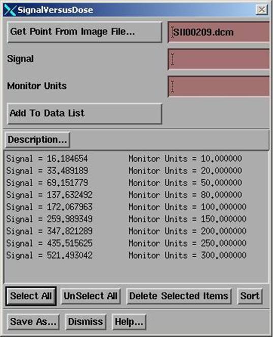
You first hit the “Get Point From Image File” button at which you will get the file selection popup shown below.

Get point from image file.

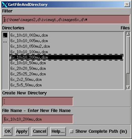
Here you can only select one file at a time. Hit the “Apply” button and use the “OK” button on the last file to take down the popup, or hit the Cancel button.

The program will read the signal value at the center of the field and write this number into the first text box as the signal value in the FitSignalDose popup shown above. You must then type in the monitor units used to expose the field. The image will also be displayed and you will also get a centering control as shown above to find the central axis if that is necessary. The signal field will update as you adjust the center.

When all fields have been entered, hit the “Fit Data” button which is described below. After fitting a straight line, save the calibration file by selecting the “Save As” button.

Files are saved to the subdirectory CalDCur.d in the data directory (located by file DataDir.loc in the program resources directory).

Fit Data

This button will bring up the curve fitting popup control. But the control will be defaulted to a linear fit. We recommend that you not change it from a linear fit. Only a linear fit can be extrapolated. Otherwise you would have to provide a zero point (which you could type in). The results of any fit will always truncate RMU < 0 to 0 and so never allow a negative RMU value.

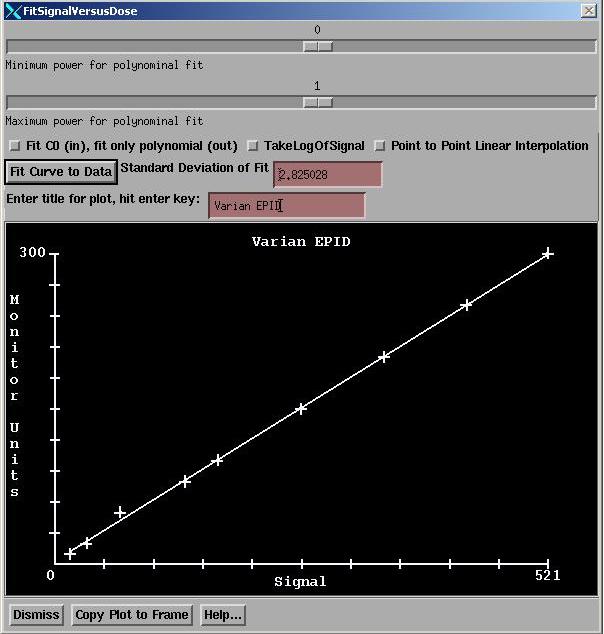
The functions of this control are described in detail in the Field Dose section of the Dosimetry Check manual. Here it is only necessary to hit the “Fit Curve to Data” button.

And you may want to enter a title for the plot.

After fitting the line, you can dismiss this popup. Then save the calibration curve.

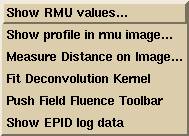
Options

Under the Options pull down are direct access to the Show Dose (RMU) function described below from the Field Dose toolbar, the show RMU profile described in the Dosimetry Check manual (Plan section), and a distance measuring tool. Be aware that the distance measuring tool will show the pixel value of the image being displayed. The pixel value is not the integrated RMU value. These tools are provided for convenience in evaluating a fluence image for correctness.

Field Dose

Access to the Field Dose toolbar as described in the Dosimetry Check manual is provided here for the convenience of using some of those functions. Only the functions under the Dose pull down will be applicable. A useful function would be to view the RMU values at different points on the field images described next. Another useful function would be to retrieve a prior fluence file.

Show Dose (RMU)

In particular, under the Dose pull down is the “Show Dose” function which can be used here to display the RMU of a converted file. Use this function to check the current calibration of a 10x10 cm field. You might want to include a 10x10 field with each case to test the stability of the EPID system for example if you are not individually calibrating images. The center of a converted test image should hold the monitor units used to make the image.

Add Fields

Another useful function is the Combine Fields function that can be used to add two or more fields together. This can also be done in Dosimetry Check by selecting more than one rmu file for a beam. If you perform this function here, you will have to formally save the result to a new file.

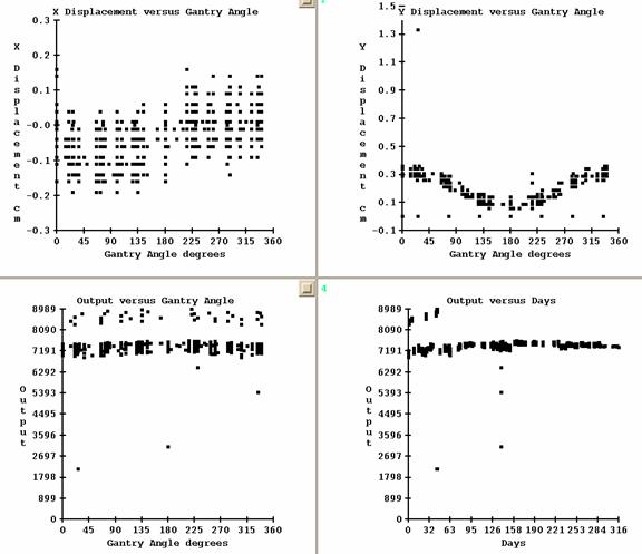
Show EPID Log Data

Use this option to display a history of the use of the calibration files. The displacement of x and y versus gantry angle will be shown. But if you had purposefully off set the EPID, that displacement will also be included in the plot. The signal at the center of the calibration field will be corrected by the inverse square law to 100 cm and plotted versus gantry angle and days since the log was started. The signal versus days might tell you some thing about the gain of your EPID over time.

Note: On and after version dated 28 Sept, 2012, the day will be the day that the calibration image was made. Prior, the day was the day that the calibration image was used.

The logged data is kept in a file called EPID.log in a path starting with your data directory (defined by DataDir.loc in your program resources directory, which is in turned defined by the file rlresources.dir.loc), the machine name, and the energy. Simply delete EPID.log if you want the log to start over again. An entry is made to the log each time images are converted, one line per calibration image:

Date calibration image made (as of 28 Sept 2012, prior was date used).

SID, gantry angle, signal at central axis, monitor units, x shift cm, y shift cm, date used.

An example of a log appears below.

Auto Report

You must select a plan for the images you are converting, and a beam in the plan for each image. For IMAT (RapidArc, VMAT), if there is more than one arc, you must have converted images for each arc. After converting all the images for all the beams in a plan, you can select to have the auto report generated. To do this, you must have selected and defined the parameters for the auto report, either from ReadDicomCheck, or from Dosimetry Check, for the plan you converted the images for, or for the plan you copied from to make the plan (trial) that you selected for the converted images to go to. The program will check if it has all the information to generated an auto report and submit a job to the batch que to do that. The program will start the batch que. The Auto Report pull down will list the plan names for which images were converted during the current run of the program, and the job will be submitted for the one that you pick.

Deconvolution Kernel and EPID Response Variations

You will need a deconvolution kernel to convert integrated fields back to in air fluence. You probably should take all your data at the same EPID SID (source image distance). There may be some variation between centers and some small changes with the calibration of the EPID. Therefore you probably should perform your own kernel fit periodically as needed. See the reference at the end of this manual. After the deconvolution of square open fields, the RMU values in the center of the fields should be the in air collimator scatter factor normalized to 10x10 time the monitor units. Generally, you can think of the rmu as an effective monitor unit normalized to the calibration field size which is usually 10x10 cm.

We define the in air scatter collimator factor Sc by the equation:

Output factor = Sp X Sc

Where Sp is the phantom scatter, and the output factor is the dose at depth of dmax. Note that measuring the Sc factor is subject to systematic error due to the need for a buildup cap, which acts like a phantom, and so is not a true in air measurement. Hence the measured Sc factor found from measurement will generally be different from that computed by dividing the measured output factor by the computed Sp factor. A pencil beam algorithm is used to compute the phantom scatter Sp, and that is divided into the measure output factor to get the in air collimator scatter factor Sc. Deconvolution of the EPID integration fields is necessary to produce the in air fluence, which is then used as input to the dose algorithm. Hence the in air fluence in the units of rmu is used to compute the dose at depth.

Lastly, it has been our experience that measured output for 2x2 fields is generally accompanied by a large uncertainty if an ion chamber is used, and generally is too small a value.

Fit Deconvolution Kernel

We now have two programs for fitting a deconvolution kernel. The original is referred to below. The second newer program was developed for the exit dose option but is equally applicable to for the case of pre-treatment images. In that case you would just fit a kernel for a set of images for 0 thickness only. The original program for pre-treatment images only is a bit tedious in that you have to select with the mouse the image file, then a corresponding point, then type in the monitor units that the image was exposed with. With the newer program you edit a file where you enter the information and then you just select to run that file. The newer program is described elsewhere under “Fit Exit Deconvolution Kernel”. The exit kernel can be use for both pre-treatment and exit images.

Hit the button provided here to get the original kernel generation tool described in the “Fitting Deconvolution Kernels for Electronic Portal Imaging Devices (EPID)” manual. But you must first convert EPID images to RMU files (Field Dose or fluence files) without the deconvolution process. Use those files along with either the output factor or water phantom scans to fit the kernel. You can fit a kernel using only a single point on the central axis which is the preferred method. To do that either use the output field factors in the machine’s data base, or you can create a profile scan file that consists of a single point for each field size. An example of a file follows below:

// Varian 2100CD 6x

/* file type: 1 = scan */ 1

/* file format version: */ 2

/* machine name: */ <*VarianStd*>

/* energy = */ 6

/* date of data: */ <**>

/* wedge number, 0 = no wedge */ 0

/* field size in cm = */ 8.00 8.00

/* field size defined at isocentric distance of machine= */ 100.000000

/* Source to Surface Distance (SSD) in cm = */ 100.0

// Here z = 0 is at SSD, negative is depth.

/* Number of scans: */ 1

/* number of points this scan: */ 1

/* x, y, z value */

0.0 0.000 -1.600 0.981

Refer to the ASCII file standard in the System2100 manual. // to end of line and /* to */ are comments which the program ignores when reading the file. Text data of more than one word must be set off with <* to *>. The value must be the dose rate in cGy/mu and must agree with the definition of the machine calibration in the calibration file. This file is to be put in the machine data directory under the proper energy directory. Note the above value is for calibration of 100 cm to surface where at a depth of 1.6 cm is 1.000 cGy/mu for a 10x10 cm field.