Deconvolution Kernel Fit Program

This program will fit the deconvolution kernel for both pre-treatment and exit dose reconstruction. The fitting routine provided with ConvertxxxxImages may still be used for pre-treatment kernels, but this routine can do both. For a pre-treatment kernel only, you would only fit for zero thickness. Since a kernel for multiple thicknesses includes zero thickness, it can be used for either case. There is little affect in taking images at different source image distances on the deconvolution kernel. However, for the exit kernel you must use a constant source image distance for all the images and with isocenter in the center of the water, for the exit kernel to work correctly with the air gap correction method.

Process

You will shoot the required images. Then run program ConvertEPIDImages as described next to normalize the images and produce an rmu file for each input Dicom file. Then you will edit the run fit file to enter the file names and list of thicknesses for your kernel. Lastly you will run program FitExitDeconvolution to accomplish the EPID deconvolution kernel fit. These steps are described below.

First shoot the images as described in the exit data needed document. Maintain a constant x-ray source to EPID distance for all the images. Adjust the couch height so that isocenter is always mid-depth. This geometry must be preserved for the air gap correction method to work correctly.

Run program ConvertEPIDImages to normalize all the images to the in air (zero thickness) calibration field (typically 10x10 cm), which can also be part of the image set. First create a new patient with ConvertEPIDImages to be used only for fitting the exit deconvolution kernel. Then select the images to be converted. You might want to do all the images for single thickness at a time, or you can do the entire set of all thicknesses.

You must then unselect using an EPID deconvolution kernel as shown below in the ConvertEPIDImages popup after selecting the Dicom image files:

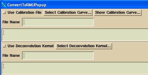
so that the only thing that happens is the 10x10 calibration image is used for normalize the output images in units of relative monitor units (rmu). Since we are fitting a kernel, the images cannot have been processed by a kernel.

Next on that same popup, you do not want a plan selected:

Leave the plan name blank. You next should consider providing meaningful names to the output files that are written out. We can suggest using a consistent convention such as: field size energy thickness. For example:

15x15_6x_05.rmu for a 15x15 field size, 6x, 5 cm thick water.

15x15_05.rmu leaving out the energy. Just create a separate patient for a different energy.

This is the only tedious part of this process, doing down the scrolled list and renaming the output files. Doing so will avoid mistakes in editing the fit run file described below and reduce the amount of editing if always using the same file name convention. And example is shown below:

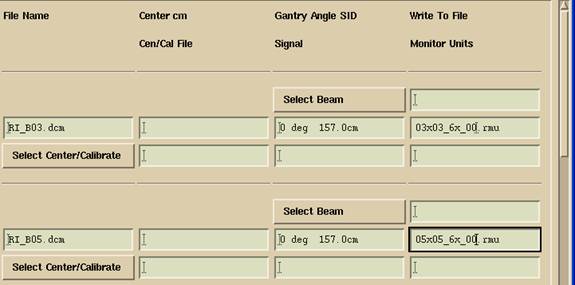
Where we have renamed the output file to 03x03_6x_00.rmu for 3x3 field size,

6x, 0 cm water thickness for the input file RI_B03.dcm.

Be sure to check that the center was found for the calibration file.

Upon converting the images, pay attention to where the output rmu files went to:

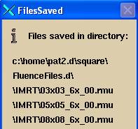
Simply copy the run fit file describe below to the same folder and edit it there.

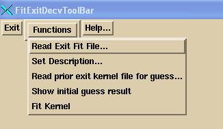
Fit Exit Deconvolution Toolbar

Run program FitExitDeconvolution.exe. The fit toolbar has only one pull down menu on it. You will first select to read in the fit file which will contain the input information directing the fit.

Run Fit File

The fit file contains all the information needed to run a fit. You must edit this file with your data. Once you have written this file, you can run it again if the need arises. This saves time from having to select a multitude of files and specifying data within a program. There should be an example fit run file in data.d\DeconvKernels.d, if not, one can be sent to you.

An example file follows below with explanations. The file follows the ASCII file standard for System2100 (see the System2100 manual). The first part of the file defines the machine name and the energy. You must also enter the SID of the EPID for the data in order for air gap distance correction to occur and be correct. The EPID is held at a constant distance with isocenter at the center of each water thickness (see data needed for the EPID exit kernel).

If narrow beam correction is on, then the file InWaterTransmissionFitnn must be in the energy directory, where nn is the energy (06 here for 6 MV).

The next field is the OCR option. For Siemens and Elekta this will be 1. For Varian probably 2 as by default Portal Vision will multiply the OCR into the integrated images. That feature can be turned off in Portal Vision in which case you would select 1 below. This choice is passed on the kernel file and can be changed there.

Next there is a description field which is passed on to the kernel file.

Next you must enter the number of fields measured. You must use the same field sizes for all thicknesses.

Collimator Scatter Factor

With each field size enter the collimator scatter factor. You can read the Sc factors from the file FieldSizeFactors_nn in the beam data directory (but see the note below about the algorithm PencilBeam or CollapsedCone). Part of a FieldSizeFactors_06 file is shown below:

Scatter collimator table for 6 MV:

For depth = dmax = 1.50 cm

Field size cm Sc Sp Scp

3.0 3.0 0.9421 0.9688 0.9127

4.0 4.0 0.9526 0.9728 0.9267

6.0 6.0 0.9747 0.9831 0.9582

You should use the Sc values from this file, not from other data, to be consistent because Dosimetry Check is computing the dose with it’s dose algorithm, and Sc must be consistent with the Sp that Dosimetry Check computes, where Sc = Scp / Sp.

If this file does not have the field size you need, make an entry in the output file for this energy and run GenerateBeamParameters to product a new field size factors file, or interpolate between the field sizes you do have. Be sure the dose rates in the output file are consistent with the calibration file.

Pencil Beam or Collapsed Cone

Because these two algorithms compute slightly different Sp factors, the program now tracks where the Sc factors came from (since Sc = output/Sp). DosimetryCheck will default the algorithm to the one where the Sc factors came from. Therefore the source of the Sc factors are specified in the below run fit file. The source is passed on to the EPID deconvoltion kernel file that is created, which in turn passes the source on in the rmu files that are created from processing the EPID image files.

Example fit run file:

Note that version file format 3 has the CC or PB source of the Sc factors in the file as shown below.

/* file type: exit dose data for fit */ 18

/* format version */ 3

/* machine name: */ <*VarianSSD*>

/* energy MeV */ 6

/* Source Image Distance of the EPID cm */ 150.00

/* Narrow Beam Correction: 0 no, 1 yes, 2 do not fit*/ 1

/* in air OCR option:

1 multiply in OCR

2 make no correction: */ 2

// Description:

<* Fit with Varian attenuation data.*>

/* Sc factors came from */ PB // CC or PB

/* number of field sizes */ 4

/* list of field sizes in order (both dimensions each) in

increasing order. Last would be 25 25 or 25 20 for example.

field size cm Sc factor */

5.0 5.0 0.9661

10.0 10.0 1.0000

15.0 15.0 1.0168

20.0 20.0 1.0260

Physical Wedges

A special note is needed here in regard to a physical wedge. Because the EPID is very energy dependent, one will not get the correct wedge factor. However, it does appear that onewill get the correct fluence slope measured with an EPID if the wedge covers the entire beam and there is sufficient common base thickness so that once the beam is hardened by that, there is little additional energy dependence on the part of the EPID. However, for a physical wedged field, a separate deconvolution kernel must be generated and used. This will require processing the wedged fields separately with a separate kernel. Trial and error will have to be tried to determine if separate kernels are needed for separate wedges (such as 15, 30, 45, and 60 degrees). Try doing one of them and see if it works for all of them.

For fitting a deconvolution kernel for a physical wedge, the images are integrated with the wedge in place for the field sizes and thicknesses. However, the images must be still normalized to the calibration image, typically 10x10 cm field size, integrated in air without the wedge. Further, for each field size, the Sc factor above must be multiplied by the wedge factor measured for that field size, and preferably measured at a depth between 5 and 10 cm. The reason for using a wedge factor measured at a deeper depth is because the wedge factor does vary some with depth, and it is better to use a number in the middle of the range of depths of interest than at one end such as dmax. Dosimetry Check does not otherwise make any correction for the change in beam spectrum after being hardened by a physical wedge.

The wedge factor is the ratio of the dose at depth for the field size with the wedge in place, to that without the wedge, typically measured with an ion chamber in a water phantom. Wedge factors change slightly with field size and with depth.

None of the above applies to a dynamic wedge. A dynamic wedge is just a sum of open fields and is no different than an IMRT beam created by a series of shaped fields. There is no beam hardening by a physical attenuator in the open fields.

Thicknesses

Next in the run file will come the list of thicknesses that were measured. You must enter the number of thicknesses that are to follow. Follow that with an entry for each thickness that specifies the total water equivalent thickness in cm, the file name for each field size and the monitor unit used for that file.

The thicknesses reported must be the total water equivalent of the total mass that is in the radiation beam, in cm. This means everything in the beam: tank bottom, supporting couch. Otherwise you will be introducing a systematic error.

The thickness must be the total water equivalent thickness that is in the beam. To measure the water equivalent thickness of non-water material, measure the transmission of the material, and then determine the amount of water that has the same transmission

(and also the ratio of thickness would be the water equivalent density. Please remember that all radiation dosimetry is based on water).

The thicknesses used do not have to be exact integers. Little error is likely to be introduced if you consider a few millimeters of plexiglass tank bottom to be water equivalent. If you have 10 cm of water in the tank including the tank bottom (for example 0.635 mm of plexiglass plus 9.365 cm of water), and the additional couch support is equivalent to 0.5 cm of water, then the total water equivalent thickness to put in the file will be 10.5 cm.

The first measurement must be for zero thickness, which means that nothing is to be in the beam (which means no couch in the beam). Otherwise you will be introducing a systematic error.

The field sizes must be listed in the same order. If you are only fitting a pre-treatment kernel, then you will only have one thickness, and that thickness will be zero. Shown below is the entry for 13 thicknesses.

/* number of thicknesses, to start with zero */ 13

// for each thickness (in order of increasing thickness) enter:

// the total water equivalent thickness in cm

// list of file names for each field size with the mu used

// for each field in same order as above!

// file name mu

0 // this first entry is nothing in the beam

5x5_00.rmu 100

10x10_00.rmu 100 // these are the file names

15x15_00.rmu 100 // each is reported to be 100 mu

20x20_00.rmu 100

5 // here is 5.0 water equivalent in the beam

5x5_05.rmu 100

10x10_05.rmu 100

15x15_05.rmu 100

20x20_05.rmu 100

Continue for all the thicknesses. In this example the last thickness was 60.0 cm.

Guess Section

The next section of the file is normally not to be disturbed. There should be no reason to edit or change this section.

It contains an initial guess for various thicknesses. The thicknesses do not have to be the same as in the above list to be fitted. Rather the program will use the closest thickness that it finds in the below list for the initial guess of paramenters when fitting a thickness specified above. The values were found below are from prior successful fits.

A iterative method for fitting parameters depends upon having a good initial guess. Once a good fit is found, those fit parameters can be used in the future as an initial guess for future problems. But getting that first guess often requires a great deal of trial and error. The file provided for this purpose has the results of a good fit for the starting guess. One also has the option of selecting an exiting or prior kernel file for the initial guesses after reading in the fit file. One can simply cycle back and read the kernel file just produced for a second go around which usually will give improved results. If a particular thickness is not fitting well, try using as a guess the parameters for the next adjoining thickness.

The guess section also specifies the number of exponentials that are to be fitted up to five. The guess sections appears as below:

// Initial guess. Closest thickness is used.

/* number of thickneses: */ 13

/* thickness cm : */ 0.000000

/* number of exponentials: */ 5

66.6448 22.9857

0.0684604 2.24048

0.00626482 0.526565

6.53152e-005 0.0650131

2.39305e-007 0.00566613

/* thickness cm : */ 5.000000

/* number of exponentials: */ 5

64.6899 23.0435

0.0691486 2.24048

0.0061963 0.557187

0.000130266 0.05228

1.79497e-007 0.00543618

and continues for all 13 thicknesses in this example file.

The last section contains information for the fitting routine:

/* min and max value for each variable

5 exponentials maximum allowed

Minimum Maximum */

1.0 200. // multiplier

10.0 100.0 // exponent

1.0e-8 100.0 // multiplier

1.0e-2 10.0 // exponent

1.0e-8 10.0 // multiplier

1.0e-3 10.0 // exponent

1.0e-10 10.0 // multiplier

1.0e-4 10.0 // exponent

1.0e-12 10.0 // multiplier

1.0e-5 10.0 // exponent

/* starting step size fraction, and stopping step size fraction, fraction of the inital guess above. Up to 5 exponentials

step stop */

1.0 0.001

For each of the up to five possible exponentials will be a list of the minimum and maximum value allowed for that exponential, in order of the multiplier followed by the exponent. This list always goes up to five pairs.

Then follows the starting and stopping fraction step size for each variable. This list always goes to ten variables, two for each exponential. The start value of 1.0 means the algorithm will begin with a step size of 1 times the initial guess. The stopping fraction of 0.001 means the algorithm will stop when the step size is 0.001 times the initial guess. Making the stopping fraction smaller will increase the number of iterations.

Set Description

You can change the description that was in the fit file.

Read prior exit kernel file for guess

You can override the values of the initial guess in the fit file by reading in an existing kernel file. This must occur after reading in the above fit file but can occur after doing a fit for a second run. Results usually improve by doing so.

Show initial guess result

This function will draw a graph for each field size and thickness showing the initial profile through the image file in the x and y directions, and the profile for both the x and y directions using the initial guess values. Plotted also will be the Sc factor times the in air off center ratio for the machine and energy selected. Ideally the processed profiles will lie on top of the off center ratio plot.

Running this option will detect any errors in the input image files before attempting a fit,

and will avoid the problem of the program ending prematurely after running for a long time because a file name was wrong some where down the list. See the below section for an example screen display.

Fit Kernel

Runs the fit. As there are separate fits done for each thickness, this could take an hour or two. When it is done the result is plotted as described above. The dotted curves should agree with the Sc factor on the central axis (see below examples). If you run this program from a command prompt window, you will see information written to standard out during the iteration process.

A kernel file is written out to the location of deconvolution kernel files. At the end of the kernel file is a report on the fit (see the below example).

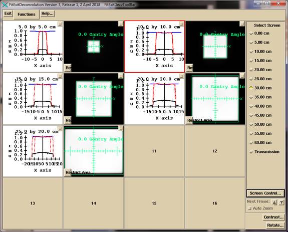
Example screen plots

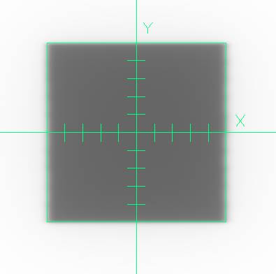
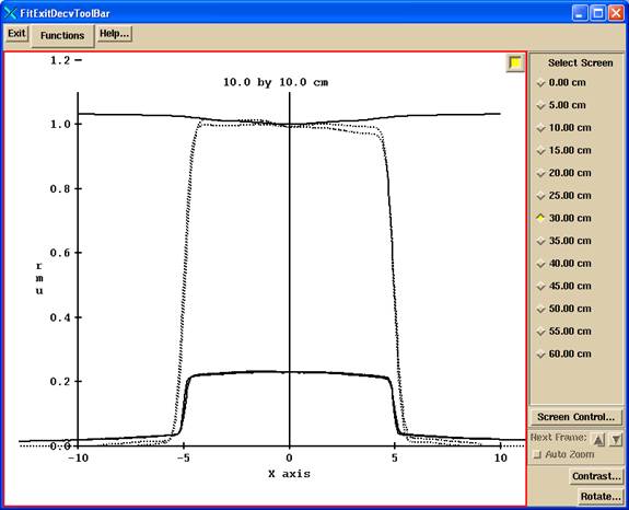
An example screen display showing the plotted results beside the image of each file after deconvolution as described above in “Show initial guess result”:

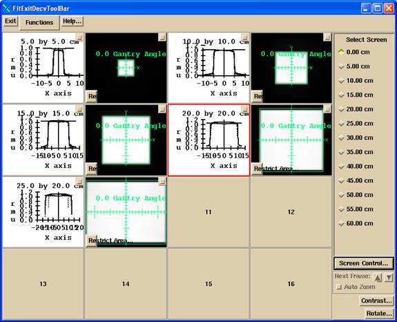
The top solid line is the Sc factor times the in air off center ratio. The two dotted lines are x and y profile after deconvolution of the input image file. The bottom solid lines are the x and y profile through the original image for the field size. Shown below is a 10x10 cm field size with 30 cm thick phantom in the beam:

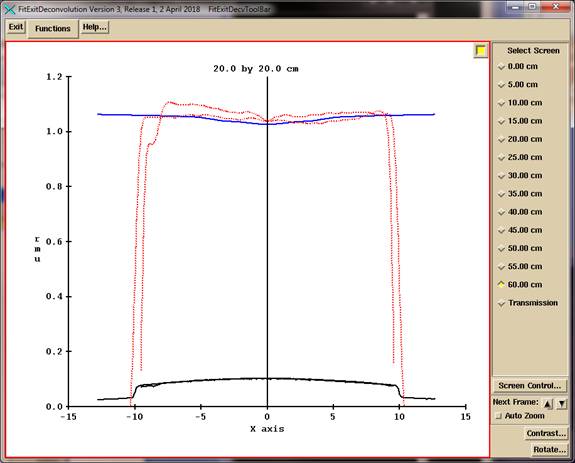
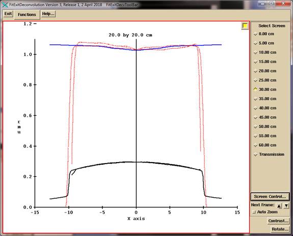
Limitation corrected for large field sizes

As the thickness gets larger and the field size gets larger, the computed profile will deviate considerably from the Sc factor times the in air off axis factor as shown below. This is presently a limitation on the method as we are assuming that the scatter is a constant across the EPID. This is not a serious limitation for small modulated fields. The EPID is energy sensitive and over responds to scatter radiation. This effect distorts the profile measured with the EPID, making the profile more rounded than it really is.

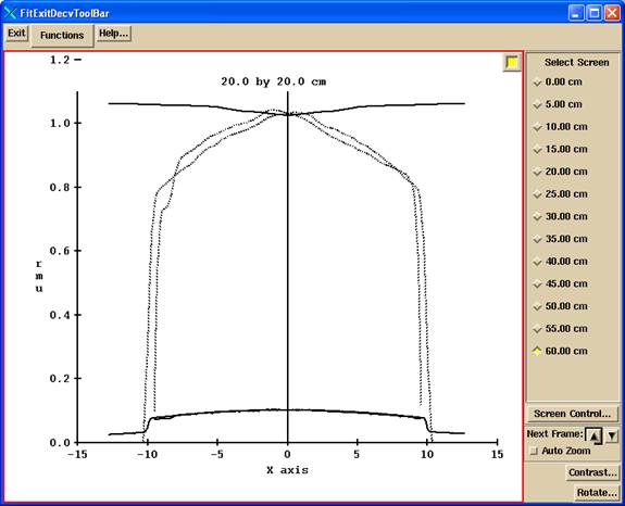
As of April 2018, the off axis transmission is fitted for a sequence of radii from the largest field size along the diagonal to correct the profiles as shown below.

This was modified February 2021 to fit a profile correction after frequency filtering, leaving the measured narrow beam transmission alone.

The program will currently write out two versions of the EPID kernel file. One with the fitted off axis transmission and one using the measured off axis transmission designated as not fitted for large field size. The second option provided if it should prove the fitted transmission is over compensating for small field sizes.

If the narrow beam flag is set to 2 in the run file, the measured is used and out putted only. Further, the fitted transmission in the EPID file can be ignored by setting the version of the file format back to 3 from 4, in which case the narrow beam transmission is read from the file in the machine folder. Otherwise the fit parameters are in the EPID file as of format version 4.

Report on Fit

The report is at the end of the kernel file, and will show the Sc factor that is computed for each field size after the deconvolution of the field image with the fitted kernel, and compared to the intended Sc factor, for each thickness. An example of the report at the end of the kernel file is shown below:

/* Report on fit

Field size response:

Field Size Raw c.a. After Sc % Ratio

cm Signal c.a. diff

Thickness = 0.000

5.0 x 5.0 0.9265 0.9665 0.9666 -0.01 1.0432

10.0 x 10.0 0.9998 1.0004 1.0000 0.04 1.0006

15.0 x 15.0 1.0417 1.0183 1.0190 -0.07 0.9775

20.0 x 20.0 1.0742 1.0300 1.0297 0.03 0.9589

Thickness = 5.000

5.0 x 5.0 0.6844 0.9668 0.9666 0.02 1.4125

10.0 x 10.0 0.7401 0.9998 1.0000 -0.02 1.3509

15.0 x 15.0 0.7821 1.0191 1.0190 0.01 1.3031

20.0 x 20.0 0.8219 1.0296 1.0297 -0.01 1.2528

...

Thickness = 50.000

5.0 x 5.0 0.0981 0.9624 0.9666 -0.43 9.8060

10.0 x 10.0 0.1147 0.9975 1.0000 -0.25 8.6992

15.0 x 15.0 0.1329 1.0290 1.0190 0.98 7.7410

20.0 x 20.0 0.1518 1.0252 1.0297 -0.44 6.7523

...

and so on for the rest of the thicknesses that were fitted. One wants to see the % difference less than 1% for all field sizes and thicknesses.

The “Raw c.a. Signal” column is of interest. It shows the normalized signal on the central axis divided by the monitor units. In doing any further test with a water phantom and square field sizes, the values there should be consistent for the same geometry (field size, water thickness, SID, and air gap). The numbers should always be getting larger as the field size gets larger. If not, the EPID is saturating.

The “After c.a.” column shows the value on the central axis after deconvolution using the fit. It should agree closely with the Sc value that the data is to be fitted to. The ratio column should start with 1.0 for 0 thickness for the calibration field size and get larger as the thickness gets larger.