The method to do this is to fit a two dimensional kernel, function of radius and transmission thickness, for fixed EPID distance and approximate phantom centered at isocenter. The kernel then accounts for both scatter reaching the EPID from the patient/phantom, and the energy response of the EPID dependence upon both scatter and the transmitted spectrum.

EPID Images for Range of Square Field Sizes

The system is designed for a fixed EPID distance. Our assumption is that a large SID will be required to clear the patient and couch. The SID of the Elekta

IviewGT EPID cannot be changed whereas the Varian can. For Varian pick an optimal distance that will be used. We have to account for scatter from a phantom to the EPID. The scatter can be expected to be a slow function of air gap and position of the phantom relative to isocenter as show below (see also figure 4, Swindell et. al., Med.Phys. Vol 23 No. 1, page 66, 1996). The EPID data is made by measuring with the isocenter always at mid-depth in the phantom (including the tank bottom) with the EPID at a fixed distance. A correction for the change in the air gap between the patient and EPID is provided for. The Elekta EPID is at about 157 cm. At this distance the EPID can measure a field size up to 25.6 cm, the Varian to 25.5 by 19.1 cm.

Patient Scatter to EPID Sensitivity to Distance

A method to provide for the change in scatter reaching the EPID from the patient with different distances from the patient to the EPID is provided. See Air Gap Correction further below. Here we illustrate the issue.

For a 30 cm thick phantom at 85 cm SSD, 10x10 cm field size we have the following data (courtesy of Sankar Andiappa, Edinburth, UK):

EPID air

SID gap 6x 10x

________________________________________

140 25 105.7 106.7

145 30 103.8 104.0

150 35 102.3 102.5

155 40 100.1 101.0

160 45 100.0 100.0

165 50 99.3 99.0

170 55 98.7 98.2

175 60 99.0 97.5

180 65 98.8 97.3

where the only the inverse square law has been applied to the EPID signal value on the central axis. If we take our EPID data at 160 cm SID, which is a 45 cm air gap, we see that the error will be 2% for an air gap of 35 cm to 55 cm. The error increases to 6% at an air gap of 25 cm. A method to provide correction for change in air gap from the assumed geometry is covered below.

Field sizes to measure.

Consider a range of fields sizes such as 4x4, 6x6, 10x10, 15x15, 20x20, and 25x25 or 25x20. Use square field sizes with the possible exception of the last one. The field sizes list above are not an exact recommendation, the point is to cover a range of field sizes. Each field size represents a sampling of the spatial frequencies involved. The software assumes all thicknesses are measured with the same field size. Stop with 20x20 if you cannot handle 25x20.

Water thicknesses needed.

Consider water thicknesses of 0, 5, 10, 20, 30, 40, 50, 60 cm with the water (phantom) covering the entire area of the beam and more. The total water equivalent thickness has to be recorded and does not have to be exact integer numbers as shown above.

The thicknesses reported must be the total water equivalent of the total mass that is in the radiation beam. This means everything in the beam: the tank bottom and the supporting couch. Otherwise you will be introducing a systematic error.

Isocenter must be in the center of the water plus tank bottom. If you have 19 cm of water and the tank bottom is 1 cm, isocenter would be at a depth of 10 cm. You may consider the tank bottom as part of the water thickness if the tank bottom material is close to water. If not, measure the water equivalency of the tank bottom and use that value added to the thickness of the water.

The equivalent water thickness of the supporting couch will have to be accounted for and included in the total water equivalent thickness that is reported in the fit run file (see Fitting the Exit Deconvolution Kernel). Use a narrow beam to measure the attenuation of the material and then water to determine the equivalent water thickness. The narrow beam transmission through water data can be used to compute the water thickness given an attenuation value. See tools.dir\ComputeThickness.exe.

The equivalent water thickness is the thickness of water that has the same attenuation value (so measure it).

The maximum thickness of 60 cm is chosen as a guess of the longest path likely to be encountered in the patient. If you stop at a smaller thickness, be aware that results will not be as accurate if a greater path is encountered in the patient. The program will use the last available thickness for the deconvolution and will not attempt to extrapolate. However, the narrow beam water transmission used for computing the attenuation through the patient is extrapolated.

The first measurement must be for zero thickness, which means that nothing is to be in the beam (which means no couch in the beam). Otherwise you will be introducing a systematic error.

The program will interpolate between thicknesses. Shown below is a plot of data for 10x10 cm field size that was taken in 5 cm increments (solid) and 10 cm dotted:

The graph demonstrates that accuracy due to interpolating over 10 cm is not lost except for the first 10 cm. Continue up to 60 cm for best results. Remember that you have to add the water equivalent thickness of what is supporting the tank that is covering the central axis in the EPID run fit file (see Fitting the Exit Deconvolution Kernel).

Sensitivity at thickness of 30 cm

Typical data attenuation measured with the EPID for 10x10 cm field size at 30 and 35 cm thickness of water is 0.2246 at 30 cm and 0.1860 at 35 cm. 0.2246/0.1860 = 1.2075 or 4.2% per cm. Consider also the British Journal of Radiology Supplement number 17, page 75, infinite SSD for 6x, with a value of 39.9 at 28 cm depth and 36.8 at 30 cm depth, for 10x10 cm field size. This computes to 5.4% per cm.

Solid Water Substitute

Solid water can be used, but you must correct for it. Consider that typical water equivalency, as quoted by Gammex, is 1.03. 30 cm of this material will be equivalent to 30.9 cm of water. At 30 cm, the difference in exit dose will change by 4 to 5% for one centimeter. Therefore if there is not a correction for the solid water, a 4 to 5% error will be built into the system. You should measure the water equivalency of the material you are using by comparing to transmission through water. You can do this by measuring the transmission (attenuation) through the solid water and comparing that to the transmission through water (with a reading slightly higher and lower than the solid water by varying the amount of water, interpolate the solid water equivalency).

Use Water

The best water equivalent material is water. If you go to www.rubbermaidcommercial.com and search for rigid liners, you can find square plastic containers of various sizes to use as a tank to hold water. You do not want something that has a mode injection dimple at the center of the bottom. We have found square sizes of 14.2 inches (36 cm) to 16.5 inches (42 cm) square, 28 to 30 inches (68 to 76 cm) high. We can recommend the RubberMaid rigid liner #3569. Plastic can be cut to be shorter. This will give you a container for water thickness of 50 to 60 cm needed for this data. You will probably need a shorter container to start with as for 5 cm of water, a 60 cm plus high container will probably not clear the accelerator head, although you could rotate the machine to point up.

Put Isocenter at mid-thickness

Given a water thickness, put isocenter at mid-depth. For example, for 15 cm of water (including tank bottom), the SSD will be 92.5 cm. Integrate the radiation exposure to the EPID for the range of field sizes and water thicknesses, changing the SSD for each change in thickness, for a known monitor unit such as 100 mu. The air gap correction assumes that the data was taken with isocenter at mid-depth. Hence you must take the images under that geometry, see below.

Figure for geometry of EPID water data.

Line Callout 2: Source of x-rays

It is important that this geometry be adhered to for application of air gap correction as described below.

Normalize all images to 10x10 cm field size for zero thickness.

Integration must also be done without the water there for the same field sizes (zero thickness above, which means there is nothing in the beam other than the EPID). Be sure to record the monitor units used. All the images are to be normalized to a 10x10 cm field in air, so if you take images on different days, you must take a new 10x10 in air for the images taken at that time.

Note that in the fitted exit kernel, the second column in the results section will show the attenuation measured by the EPID. This data can be helpful for checking for errors by comparing to other such measurements.

Procedure

Use water tank or solid water (but correct). No void on central axis please.
Fill to different depths in increments to 60 cm as above.
For each depth, put isocenter at center depth.
Put the EPID at 157 cm or there about (One should always use this distance when doing patients. Consider the distance that will be used with actual patients). Record the distance used.
For range of field sizes (up to the maximum that the EPID can handle at the distance).
Integrate the EPID image for 100 mu.
Integrate the same field sizes without anything in the beam.

Table for measured images data

Distance to EPID ________________ cm

Field size	MU	Thickness	File name

Air Gap Correction

Additional data is needed to correct for geometry which deviates from isocenter at the center of the patient. As shown above, the dose at the EPID has some sensitivity to changes in the exit surface to EPID distance (air gap). However, errors are more significant for larger field sizes. A method is provided to make corrections. By normalizing data for each field size, we are employing differences rather than absolute values for the correction method. The differences are less dependent upon a particular machine, so we can use one set of data on more than one machine.

EPID Images to Take

The data is to consist of images taken for a range of thickness, field size, and air gap. The same set of field sizes must be used for all thicknesses, but the air gaps can be different. We can suggest 5x5, 10x10, 15x15, 20x20 field sizes for thicknesses of 5, 10, 20, 30, 40, 50, and if possible, 60 cm of water. The air gaps to start from the largest possible to the smallest for any field size, but need not be the same for all thicknesses and field sizes. Below will describe how the data will be fitted.

Geometry

The above geometry is necessary for those EPID kernel images and is assumed here in applying the air gap correction by use of the equation shown later below.

Air Gap Correction Run File

Take images and keep a running log of:

the image file name, field size, thickness, air gap, and monitor units.

This log can go directly into a text file which will serve as the run file for generating the air gap correction table. An example run file follows where … designates continuation of listing integrated image files:

/* file type: Exit air gap correction run fit file */ 22

/* format version */ 1

/* energy MeV */ 6

/* machine directory name */ <*VarianSSD*>

DIRECTORY // sets a subdirectory for all future files.

Thick10.d

CALIBRATION // specifies calibration file for all following files

/* 10x10 in air calibration file name, monitor units */

10x10_6xcal_03.28.12.dcm 100

/* file name field size, thickness cm, air gap cm mu */

12010x106x.dcm 10 10 10 15 100

12020x206x.dcm 20 20 10 15 100

…

Fit Air Gap Correction

Program FitAirGapCorrection will sort the files by thickness, field size, and air gap. It will then fit a 2^nd order polynomial to the data for each field size and thickness. The curve will be extrapolated to zero field size and extended in the other direction. Once the minimum of the parabola is reached, the curve will just extended at that minimum.

Example Air Gap Fitting

Below is an example plot for 30 cm thick, 20x20 cm field size:

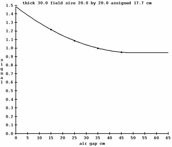
In the above plot, notice that the plot is extrapolated to zero air gap on the left, and is extended on the right after reaching a minimum.

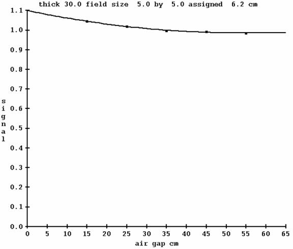
Another example below is given for a 5x5 cm field size. Notice that the change with air gap is much less.

Air Gap Fit Normalization

For any given thickness, the curve is normalized to 1.0 for the air gap from the equation:

Air gap = EPID SID – (100.0 cm + 0.5 x thickness )

For 30 cm thickness and 150 cm SID, the normalization is to an air gap of 35 cm. In application, the data is renormalized to what ever SID was used for the EPID kernel data. It is therefore important that the EPID kernel images be taken so that the above equation gives the correct air gap for a given thickness.

Application to Clinical Exit Images

On a pixel by pixel basis, given the air gap, thickness, and field size, a correction factor is interpolated from the three dimensional air gap correction table and applied to that pixel value. The field size must be generated by some metric that will account for the amount of scattering from the radiation field since modulated fields are not open square and rectangular fields. For each field, the maximum intensity is found, and all other pixels are divided by that. The pixels are then all summed up, multiplied by the area of a pixel, the square root taken, and demagnified to 100 cm.

In the two above examples the program computed 6.2 cm for the equivalent square of a 5x5 and 17.7 for the 20x20. While something of a loose metric, it provides a means of a common measure for all radiation fields.

Narrow beam transmission through water

The purpose of the data is to account for the transmission through water and how the transmission changes off the central axis for a narrow beam.

However, as of April 2018 and revised Feb 2021, the transmission off axis can be mitigated from the EPID data in the deconvolution kernel by program FitExitDeconvolution which can fit a post deconvolution profile correction (see the Exit White Paper). Hence measuring the transmission on the central axis would most likely be sufficient.

For best results, the narrow beam transmission should be measured on the central axis and used. FFF will be different from FF.

To measure on the central axis, you need only put an ion chamber below a water tank on the central axis with a good air gap between the bottom of the tank and the ion chamber, set a small field size, and measure for a range of water thicknesses. Use the same software program FitTransData for the single radius of zero to fit the exponential parameters.

This data is not expected to change significantly from one machine to another among the same model machine, and so generic data measured once is probably going to be sufficient. Since the EPID deconvolution kernel is fitted using this data, any absolute errors will cancel out.

Off axis attenuation

Typical results for 6x at 30 cm thickness with a flattening filter are:

At thickness of 30 cm (along the slant ray):

Radius cm Attenuation % Difference

at 100

0.0 0.2176 0.00

2.5 0.2157 -0.87

5.0 0.2121 -2.54

7.5 0.2088 -4.08

10.0 0.2044 -6.07

13.0 0.1985 -8.80

15.0 0.1939 -10.90

18.0 0.1866 -14.25

!5x at 30 cm thickness:

At thickness of 30 cm (along the slant ray):

Radius cm Attenuation % Difference

at 100

0.0 0.4129 0.00

2.5 0.4104 -0.62

5.0 0.4069 -1.47

7.5 0.4020 -2.66

10.0 0.3974 -3.77

12.5 0.3916 -5.17

15.0 0.3854 -6.66

17.5 0.3797 -8.05

Measure approximation to zero field size.

Transmission is the ratio of a measurement with the water in the beam divided by the measurement without the water. The geometry is picked to come close to measuring zero field size transmission. A large air gap between the water and ion chamber will eliminate some scatter from the water. Room scatter to the ion chamber will cancel out. Measure with a large air gap for a NARROW beam just big enough to cover the ion chamber (which will need a build up cap) without introducing uncertainty from positioning.

Measure along diagonal.

No longer needed after April 2018. But if still measuring off axis:

Measure narrow beam transmission through water along the diagonal of a field. At 100 cm this is to the corner of a 40x40 field, which is 28.28 cm from the center, 15.79 degrees with the central axis, or the tangent is 0.2828 (radius at 100 divided by 100), provided that the field is a square. Measure about every 2 degrees starting with the central axis to a corner which works out to about 3.5 cm along the diagonal at 100 cm. However, on most machines the 40x40 field is really round. In that case going to a radius of 20.0 would be sufficient, and every 2.5 cm along the radius would most likely be sufficient.

Because the data with the water in the beam is divided by the measurement without anything in the beam, room scatter will cancel out.

Depths to use.

Depths in increments of 5 cm would be sufficient resolution most likely, out to 40 cm at least, but ideally to 60 cm of water. However, the program fits a sum of exponentials to the data and so it can be extrapolated.

Use narrow water container.

If still measuring off axis:

This could be done by purchasing a plexiglass cylinder. One can rotate the gantry and translate the cylinder. The cylinder must be parallel to the diverging ray. The field could then be left wide open, or alternately have the MLC create a small field moving with the cylinder. One wants to simulate as small a beam as practical to cover an ion chamber with a brass buildup cap. And to also use as large an air gap from the exit surface of the phantom to the chamber as practical. The actual distance to the chamber does not matter as long as the measurement series includes zero material in the beam. With this geometry, the height of water would be along the diverging ray.

Use MLC to collimate narrow beam.

This could also be done with a water tank and using the MLC to cone down to the chamber, but one would be limited to 40 cm thickness most likely. The gantry can be left stationary with the MLC moving a small field along a diagonal and the chamber moved to match. In this geometry the water height is measured along the central ray and the slant height can be computed. The jaws or MLC will be needed to make a small field that will advance long the diagonal of the 40x40 cm field.

Procedure

Use water tank or narrow cylinder.
Fill to different depths in increments of 5 cm.
Put ion chamber under the water tank with build up cap as far as possible below the water tank (or you can shoot up instead). You will need a build up cap.
Set small field size with the MLC (as small as is practical if not using a narrow column of water).
Expose chamber on the central axis.
If still measuring off axis: move the chamber and field along a diagonal, always with the same small field size, in increments of 2.5 cm along the diagonal at 100 cm.
Include a measurement with nothing in the beam.

Format for narrow beam transmission through water data

State whether the water thickness is slant along the ray or along the central axis:

	Distance from central axis at 100 cm, to corner of 40x40 field in increment of 2.5 cm to 20 cm along the diagonal.
Water thickness Cm	0.0	2.5	5.0	7.5
0
5
10
15
20
30
40

thickness	10.0	12.5	15.0	17.5	20.0
0
5
10
15
20
30
40

Since a 40x40 cm field is typically a round field with a radius of 20 cm, the data needs only go to a radius of 20 cm. So an increment of 2.5 to 5.0 cm will do.

The thickness is the vertical depth of the water. The actual path, being on a slant, will be more.

Figure for geometry of narrow beam measurements.

(using the MLC to collimate a narrow field)

Record the dose rate in cGy/mu at for each of the field sizes above at the calibration depth of _______ cm, for SSD of ___________ cm:

Field size
cGy/mu

Record the calibration condition of the accelerator:

Field size	SSD	depth	Dose rate cGy/mu