Fit Transmission Data
13 August 2010
Introduction
The utility program FitTransData.exe is to fit a sum of exponentials to narrow beam transmission data measured on and off the central axis. The fit is for the purpose of interpolating between thickness points and extrapolation beyond the range of thickness, although the range should include the clinically relevant range for greater accuracy. This data is optional but recommended for greater accuracy of reconstructed dose when processing exit images back to in air x-ray fluence images.
Input File
The measured data is to go into the file with the name InWaterTransmission06 and that file is to go in the energy directory for the particular machine. The file follows the ASCII file standard of System 2100. An example file follows:
/* file
type */ 17
/* file
format version */ 1
/* transmission through water */
/* energy
Mev */ 6
/*
distance to detector cm */ 230.7
//
October 2009, Varian
// off
axis distance at detector distance
//
equavilent water thickness (2 cm acrlic + water) transmission //value, 2 cm acrylic = 2.274 water page 177 Hendee
/* number
radii */ 8
/* number
of depths */ 7
/* depth
is along central axis: 1, along slant ray 2 */ 1
//depth
cm radii cm at
100 cm
0
2.5 5.0 7.5
10.0 13.0 15.0
18.0
0 487.8
498.6 513.5 522.8
531.4 547.6 559.2
574.7
5.274 369.8
376.3 385.8 391.0
395.5 403.9 411.1
418.4
10.274
282.1 286.1 293.1
297.1 298.2 303.7
308.4 311.8
15.274
219.2 222.7 226.7
228.2 228.7 231.6
233.4 233.5
20.274
169.9 172.1 175.5
177.6 176.8 178.4
177.9 176.8
30.274
104.3 105.9 107.1
107.0 106.0 104.8
104.3 102.7
40.274 66.6
67.6 68.1 67.6
66.8 66.2 65.2
63.3
The depth range should cover to the chosen maximum depth. Each column is the measured transmission for the ray that intersects the plane at the given radius at 100 cm, and need not be normalized the same. The transmission is for a narrow beam to approximate the transmission along a primary ray. A large air gap should be used to improve this approximation to minimize the scatter radiation that would reach the detector from the phantom. Thicknesses must be water equivalent.
Pick Accelerator
Upon running FitTransData, the first toolbar will require the user to pick the accelerator and energy.

Then hit the continue button. The program will attempt to read the above file and if it cannot find it will display the message:
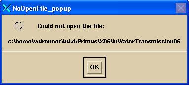
You can then select to alternately read in a file that might be somewhere else on the Fit Transmission Toolbar.
Fit Transmission Toolbar
There are three selections on the Functions pull down:
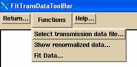
Show Renormalized Data
The “Show renormalized data” will simply rewrite to a file and display the data normalized to 1.0 for zero thickness and correct the thicknesses to be along the slant rays if not already measured do:
Data from file: InWaterTransmission06
Written to file: c:\home\tmp.dir\TransmissionData.txt
Corrected to slant
thickness.
Radius at 100 cm
0.00
2.50 5.00 7.50
Thick
Value Thick Value
Thick Value Thick
Value
0.00
1.00000 0.00 1.00000
0.00 1.00000 0.00
1.00000
5.27
0.75810 5.28 0.75471
5.28 0.75131 5.29
0.74790
10.27
0.57831 10.28 0.57381
10.29 0.57079 10.30
0.56829
15.27
0.44936 15.28 0.44665
15.29 0.44148 15.32
0.43650
20.27
0.34830 20.28 0.34517
20.30 0.34177 20.33
0.33971
30.27
0.21382 30.28 0.21239
30.31 0.20857 30.36
0.20467
40.27
0.13653 40.29 0.13558
40.32 0.13262 40.39
0.12930
Radius at 100 cm
10.00 13.00 15.00 18.00
Thick
Value Thick Value
Thick Value Thick
Value
0.00
1.00000 0.00 1.00000
0.00 1.00000 0.00
1.00000
5.30
0.74426 5.32 0.73758
5.33 0.73516 5.36
0.72803
10.33
0.56116 10.36 0.55460
10.39 0.55150 10.44
0.54254
15.35
0.43037 15.40 0.42294
15.44 0.41738 15.52
0.40630
20.38
0.33271 20.44 0.32579
20.50 0.31813 20.60
0.30764
30.42
0.19947 30.53 0.19138
30.61 0.18652 30.76
0.17870
40.47
0.12571 40.61 0.12089
40.72 0.11660 40.92
0.11014
Fit Data
Upon selecting the Fit Data function, the program will fit each column to a sum of exponentials. The program will write a report file out, shown below, which you can use to assess how well the fit is.
Data from file: InWaterTransmission06
Written to file: c:\home\wdrenner\tmp.dir\FittedTransData.txt
Corrected to slant thickness.
Radius at 100 cm
0.00 2.50
Thick Value Computed Difference Thick Value Computed Difference
0.00 1.0000 1.0000 0 0.00 1.0000 1.0000 0
5.27 0.7581 0.7548 0.003294 5.28 0.7547 0.7521 0.002579
10.27 0.5783 0.5807 -0.002426 10.28 0.5738 0.5771 -0.003311
15.27 0.4494 0.4490 0.0003562 15.28 0.4467 0.4453 0.001327
20.27 0.3483 0.3490 -0.0007468 20.28 0.3452 0.3458 -0.0006047
30.27 0.2138 0.2148 -0.001021 30.28 0.2124 0.2129 -0.0004971
40.27 0.1365 0.1360 0.0005508 40.29 0.1356 0.1353 0.0002684
Radius at 100 cm
5.00 7.50
Thick Value Computed Difference Thick Value Computed Difference
0.00 1.0000 1.0000 5.96e-008 0.00 1.0000 1.0000 0
5.28 0.7513 0.7493 0.00204 5.29 0.7479 0.7470 0.0009072
10.29 0.5708 0.5729 -0.002113 10.30 0.5683 0.5694 -0.001144
15.29 0.4415 0.4406 0.0008824 15.32 0.4365 0.4366 -7.498e-005
20.30 0.3418 0.3411 0.0007079 20.33 0.3397 0.3369 0.002819
30.31 0.2086 0.2090 -0.0004396 30.36 0.2047 0.2052 -0.0005369
40.32 0.1326 0.1326 6.174e-005 40.39 0.1293 0.1295 -0.0001674
Radius at 100 cm
10.00 13.00
Thick Value Computed Difference Thick Value Computed Difference
0.00 1.0000 1.0000 5 .96e-008 0.00 1.0000 1.0000 0
5.30 0.7443 0.7441 0.0001428 5.32 0.7376 0.7387 -0.001156
10.33 0.5612 0.5651 -0.003894 10.36 0.5546 0.5573 -0.002686
15.35 0.4304 0.4315 -0.001093 15.40 0.4229 0.4229 2.179e-005
20.38 0.3327 0.3316 0.001145 20.44 0.3258 0.3232 0.002626
30.42 0.1995 0.2002 -0.000766 30.53 0.1914 0.1934 -0.002015
40.47 0.1257 0.1253 0.0004065 40.61 0.1209 0.1204 0.0005001
Radius at 100 cm
15.00 18.00
Thick Value Computed Difference Thick Value Computed Difference
0.00 1.0000 1.0000 0 0.00 1.0000 1.0000 0
5.33 0.7352 0.7353 -0.0001906 5.36 0.7280 0.7292 -0.001125
10.39 0.5515 0.5522 -0.0007074 10.44 0.5425 0.5432 -0.0006139
15.44 0.4174 0.4171 0.0002851 15.52 0.4063 0.4070 -0.0006846
20.50 0.3181 0.3172 0.000936 20.60 0.3076 0.3071 0.0005405
30.61 0.1865 0.1881 -0.001553 30.76 0.1787 0.1795 -0.0008225
40.72 0.1166 0.1162 0.0004396 40.92 0.1101 0.1097 0.000406
Average |difference| = 0.0035754
Average variance = 1.24744e-005
Fit File
The results of the fit are written to file InWaterTransmissionFit06 in the selected beam data directory. An example follows:
/* File type, 110 = in
water transmission fit: */ 110
/* file format version: */
1
/* machine directory name:
*/ <*Primus*>
/* nominal energy MeV */ 6
/* number radii: */ 8
/* number of variables per
radii: */ 8
// fit parameters
(multiplication factor, exponent) in order:
/* tangent of radius: */
0.0000 // Parameters:
0.78796 0.0599683
0.16061 0.0351419
0.0477834 0.0182022
0.00364716 0.000232138
/* tangent of radius: */
0.0250 // Parameters:
0.79023 0.061081
0.162944 0.0340008
0.0450299 0.01496
0.00179578 0.000123193
. . .
/* tangent of radius: */
0.1800 // Parameters:
0.911175 0.063133
0.0596556 0.0275217
0.0287254 0.00748195
0.000443495 0.0001
/*average variance of the
fit = */ 1.24744e-005
<*05-May-2010-11:21:58(hr:min:sec)*>
/*
At thickness of 30 cm (along the slant ray):
Radius cm Attenuation % Difference
at 100
0.0 0.2176 0.00
2.5 0.2157 -0.87
5.0 0.2121 -2.54
7.5 0.2088 -4.08
10.0 0.2044 -6.07
13.0 0.1985 -8.80
15.0 0.1939 -10.90
18.0 0.1866 -14.25
*/
This file will be referenced when needed by the EPID deconvolution kernel fitting program and the convert image programs when processing exit images. The attenuation at 30 cm depth is reported for information.
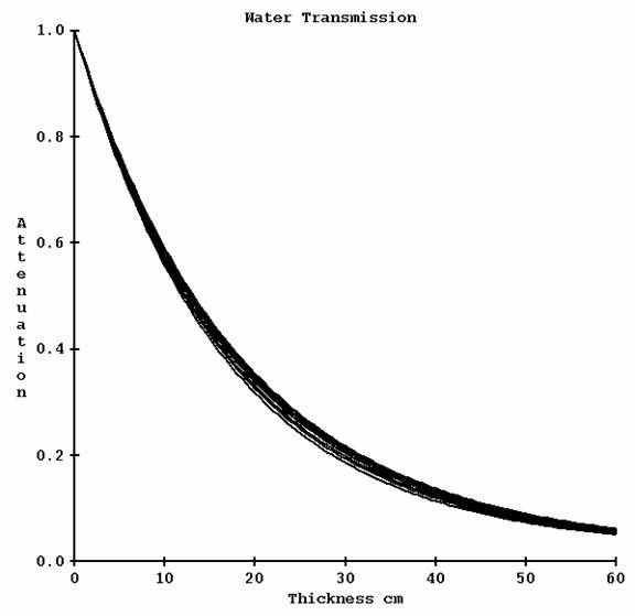
Graph of Fit
Lastly the program will graph the fitted curves for you.