This manual describes using Dosimetry Check to verify an IMAT course of treatment such as RapidArc (from Varian) or VMAT (from Elekta). In order to reconstruct the dose to the patient, the arc is simulated with a series of closely spaced stationary fields. This will require the integration of the rotating beam at periodic closely spaced angles, which probably should be no more than 10 degrees apart. As an alternative one could integrate for the entire arc and do a comparison of a fixed beam for the composite dose.

Varian Portal Vision

We have been successful in using Aria and Mosaic to measure the fluence for RapidArc rotations, with integrated files produced about every 5 degrees. Alternately one could manually stop the integration as described below. Here we describe continuous acquisition. In this mode the gantry angle reported is close enough to being the center angle.

Continuous Acquisition Mode for Portal Vision

1) Log into Eclipse/Administration

2) Under lower tabs, go to “Templates & Processing”

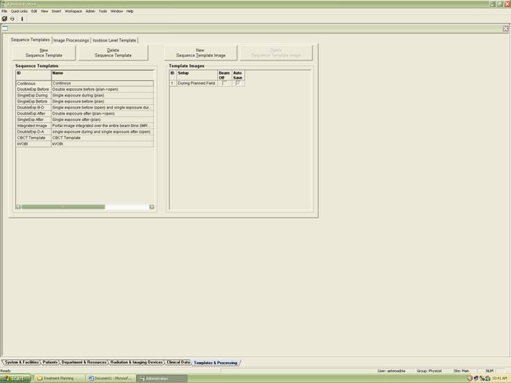
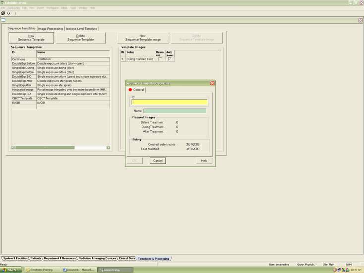
3) Click on “New Sequence Template” on the left. Enter the desired name, only yellow fields are mandatory. Click OK

4) As the new sequence template appears on the left hand list, click on it to highlight the options available to you on the right.

5) Click on “New Sequence Template Image” of the new technique and choose “New Sequence Template MV Image”. Under the “General” tab, choose during and click off the “Beam Off” option.

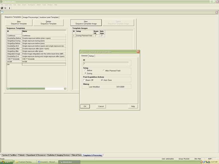
6) Under the “Setup” tab click on continuous option.

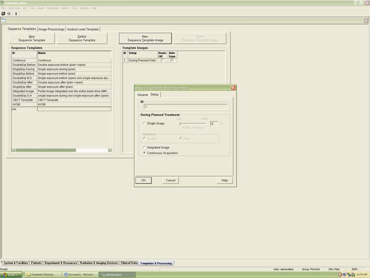
7) Click OK, save and exit.

8) In RT Chart, whenever scheduling plans under the “Schedule” tab, make sure to choose this new technique for your Rapid Arc plans with Dosimetry Check.

Time Gap Between Images

In continuous mode there may be some small time gap between images. Measurement showed a loss of 1% of the integrated radiation (as described below). This can be demonstrated by making a RapidArc measurement in continuous mode and adding up all the integration files, and then making a single integration for the same arc for the same total monitor units. However, another issue may be a change in EPID gain between continuous mode and IMRT mode.

Accordingly we have provided a mechanism for correcting for any discrepancy between continuous mode and a single integration of the entire arc. This will require a second “single” integration of the arc and is described in a section later below.

However, an analysis is provided below for this one issue.

Analysis of time gap

Let Rc be the ratio of the value for a single integration for a point in the field divided by the sum of the fields measured in the continuous mode for the same point within the field. By point we mean a location within the plane of the measured fluence, which in Dosimetry Check is in the units of the rmu (relative monitor units).

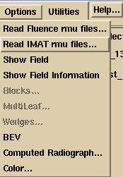
A convenient method to add up all the fields measured in continuous mode is to use the adding feature of non-IMAT IMRT fields in Dosimetry Check. Simply make a bogus plan and a bogus beam, and from the Beam Toolbar under the Options pull down, select “Read Fluence rmu files”. Select all the IMAT files and the program will add all of them up into a single image file. Then from the Evaluate pull down on the Plan Toolbar select the Show RMU Value tool to get the rmu value at a point within the fluence field. Make another beam and use the same method to get the value from the single integrated field.

The single integration will have recorded all the radiation. We will consider the time for the individual integrations in continuous mode and any time gap between those images. The total radiation measured by the single integration may be expressed as the equivalent time sequence:

Total rmu = (n t_i + (n-1) t_g) dr

And the rmu measured by the sum of the individual fields measured in continuous mode will be:

Measured rmu = (n t_i ) dr

where t_i is the time for the individual integrated fields integrated during continuous mode, and t_g is the gap time missed between integrations. The term dr is the dose rate, which for our purposes here will be approximated by the assumption of being constant. Likewise we will assume that t_i and t_g are constant. These are reasonable approximations for deriving a small correction. However, if the integration time in continuous mode is changed, then a new measurement will have to be made.

From our measurement of the total rmu value by doing a single integration for the same beam, and the rmu found from summing the individual fluence fields measured in continuous mode, we have a correction factor for n such measured fields, and is simply:

Rc = Total rmu / Measured rmu

where Rc > 1 by necessity. We simply scale everything up by multiplying everything by the factor Rc. The effect of the missing radiation of the order of 1% or even 5% is going to have a negligible effect on the dose distribution. This factor can be applied in the Fractions/Normalization field on the Plan Toolbar. Any number entered there multiplies all results.

From the above we have:

Rc = (n t_i + (n-1) t_g) dr / (n t_i) dr = 1 + [ (n-1)/n ] t_g/t_i

Solving for t_g/t_iwe have:

t_g/t_i = (Rc – 1) n/ (n-1)

So once we have a measurement for n, we can solve for t_g/t_i and then apply the above equation for Rc for any other n.

Manual stopping for integration

The RapidArc may be broken into sub-arcs of the order of 10 degrees either manually or in an equivalent selected mode. If done manually the angle of the center of each sub-arc must be recorded.

Inclinometer

This can be done with a provided inclinometer and program. There must be a clear stop between each image recorded by the inclinometer program. Three successive angle readings are checked, by default every 0.25 seconds, and by default the angle should not change by more than 0.25 degrees. When the gantry moves more than 0.25 degrees, the gantry is considered to be rotating again. The angle criteria and time can be adjusted in a data file in the program resources directory shown below. The inclinometer file may be copied into the same directory with the image files and automatically read, or selected manually.

InclinometerAngle.dat

The file InclinometerAngle.dat in the program resources file may be optionally used to change the default settings used for this process:

/* file format version */ 1

// File to put tolerance angles for use of the inclinometer.

// Time between angle measurements when not writing a file in millisec

500

// Time between angle measurements when writing a file

250

// minimum change in angle (degrees) for accelerator to have started

0.25

// maximum change in angle for accelerator to have stopped

// rotating for three angles in a row:

0.25

Gantry Angle File

If the inclinometer program is not available, then the angles must be recorded manually and written to a file. The file name is FileGantryAngles.txt and has the format of the image file name, or a unique portion of the file name, followed by the gantry angle, as shown in the example below:

SID00949 283.6

SID00950 274.15

SID00951 265.15

SID00952 255.75

SID00953 245.7

954 236.05

955 226.05

Elekta IviewGT

With Elekta VMAT, the IviewGT system can integrate periodically during the rotation. However, the gantry angle is not recorded for each sub-arc that is integrated.

XML log file

The gantry angle can be recovered from a log file of dose rate versus time and gantry angle versus time that can be generated by the control console of the accelerator. The file produced is of type extension .xml. Run program IviewToDicom, select VMAT, and pull in the integrated images. Put the xml file into the same directory where the Dicom files were written to. The xml file can have any name but must end in .xml. If more than one file is there, the newest one is used.

Inclinometer Program

We have developed software to gather angle versus time with an inclinometer and a supplied program if that should be preferred.

ConvertIMATImages

Run program ConvertIMATImages. This program is identical to ConvertEPIDImages except for a few details. Only select the files that belong to a single arc. If there is more than one arc, then you must do each group separately.

In the directory where the image files are, for convenience, you can put the 10x10 calibration file. Include the letters “cal” or “CAL” in the file name and the program will automatically pick up the calibration file. Otherwise you can use the Center All/Cal All button to select the calibration file. Files ending in .txt or .xml will be ignored for the purpose of reading in an integrated image but otherwise used as described above. We presently are not correcting for any shift in the EPID during rotation.

After selecting the Dicom integrated files, you will get the convert popup shown below:

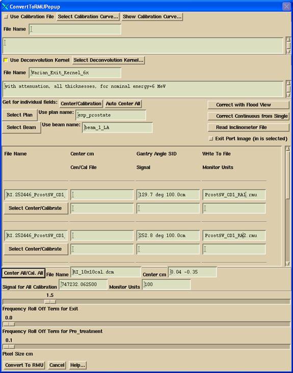
If you have downloaded the plan to the selected patient, then the list of plans is available on the option menu shown. Select the plan and then select the beam the measured files are for. The selected beam will appear in the text field to the right of the option menu for the list of beams. You can further modify the name if there is a reason to or type in a different beam name. However, Dosimetry Check will look for an exact match. If there is not an exact match, you will have to select the rmu files in Dosimetry Check for the beam. The path for storing the processed files is:

patient_name -> FluenceFiles.d -> plan_name -> beam_name -> IMAT -> all rmu files for an arc.

The file names of the rmu files do not matter here since you will typically select all the files in this folder.

Note also that the gantry angle for each file is shown. You should review these angles for correctness. The angle displayed will be in the coordinate system of the accelerator as defined by the Geometry file in the machine’s data directory. The angles can be edited, but each text field must contain and start with an angle. The arc will be simulated by a fixed beam at each of these angles using the corresponding fluence field developed here. The angles of rotation of the beam from the plan are ignored.

Flood View Correction

Providing a flood view correction is described in the ConvertEPIDImages manual. It would seem unlikely that you would have to off set the EPID for IMAT.

Combining Images Close in Gantry Angle

Images within a specified gantry angle spacing will be combined into a single image with the average angle assigned. The default angle spacing is 5 degrees. The angle spacing may be set in the file IMATGantryAngleSpacing in the program resources directory. An example file is shown below:

/* format version */ 1

// file to default minimum spacing of IMAT images by gantry angle in //degrees

This will occur before the images are processed. Images may also be combined after processing on the beam toolbar as described under “Select Imat Images Spacing” in the Beam section of the Dosimetry Check manual.

Correcting a Continuous Integration

You can renormalize the files resulting from a continuous “cine” mode integration to agree with that of a single integration of the entire arc. This might be needed if the gain of the EPID is different in continuous “cine” mode or there is some loss of radiation measurement between images. However, information has been received from Varian on how to assure the same gain in continuous and IMRT mode.

Correct with calibration image taken in continuous mode

However, if it can be demonstrated that generating the calibration field in continuous “cine” mode produces the same correction factor, you can instead generate the calibration field in cine mode, by which you will produce multiple image files. This must be for a known total monitor unit. You can then select all the files produced in cine mode

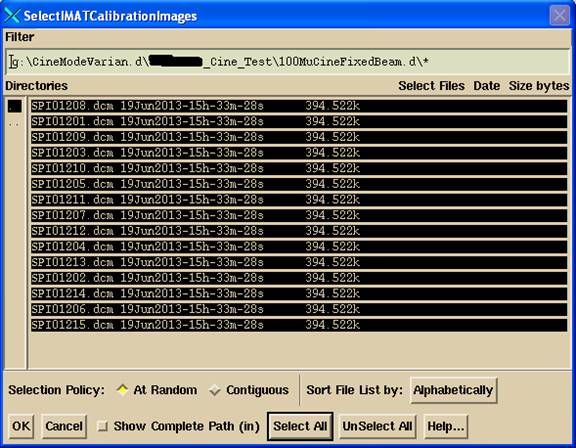
and type in the total monitor units, 100 in the above example of the ConvertToRMU popup.

The program will add up all the files you select at one time from the file selection dialog. It is assumed that the EPID is not moved during the integration relative to the source of x-rays. The files are simply summed into one calibration image. Whether this procedure will work will have to be determined by the user, including what monitor unit to use for the total to generate the calibration images.

Correct with second integration of IMAT images

The below may otherwise be used if the calibration image is generated in the same mode used for the integration of the arc into a single image. That is, integrate the arc twice, once in continuous mode and once in single integration (IMRT) mode. Use the single integration mode image to correct the cine mode images.

Hit the “Correct Continuous from Single” button, and then select the single integration for the same entire arc. A single correction factor will be computed from comparing the single integration to the sum of the continuous integrated files. The ratio will be computed for all pixels >= 0.25 of the maximum pixel value in each image, between the pixel value from the single image divided by the value from the sum for that same pixel location. The average of the ratios will be computed along with a standard deviation with the result displayed in a popup:

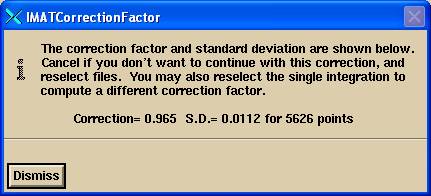
Where here for what ever reasons the sum of the continuous had a greated value than the single integration. The correction value shown is simply used to multiply all pixels of all images. Since any missing radiation will be a small percentage, its effect on the over all dose distribution will be negligible once the dose is scaled accordingly.

If you elect to not do a correction, than cancel the popup and reselect the files to be converted.

If you establish that the correction is always the same, you can always enter this factor into the normalization/number of fractions text box on the Plan toolbar of Dosimetry Check. If the number of fractions is greater than one, just multiple that number by this factor.

For the Exit Dose Option, you might have to do the second integration on a different day.

Inclinometer

The output from the inclinometer can be use to assign angles to individual Dicom RT image files. Either copy the inclinometer file into the same folder that the image files are in, or manually select the file to use. The file name must begin with IA_ and end with .txt for the file to be automatically found in the images folder. You can also select the file to be read in.

Exit Port Image

Select this toggle button in if the images were taken during patient treatment. See the separate manual on the Exit Dose Option for more details. Basically, you must select the correct plan and beam, and in Dosimetry Check the correct body outline and CT number to density file must have been selected.

Correction for TrueBeam IPS Continuous Mode for RapidArc

Varian version 2.0 for integration of images during RapidArc has two errors in the exported Dicom RT file: The gantry angle is reported for the kVp imagier instead of the MV imager, and so is off by 90 degrees, reporting 270 instead of 0 (or 360). The SID is incorrect. Varian version 2.5 MR1 has fixed this problem and you need do nothing here.

Images taken for Rapid Arc are to be taken in IPS Continuous mode (see note following below). There will be one image per frame, so there will be a large number of image files. This program will combine images into groups as specified in the program resources file IMATGantryAngleSpacing as explained above.

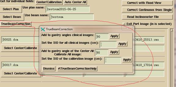
A method is provided here to correct the gantry angle and SID. As was not shown above, there is an extra button added to the convert popup called TrueBeamCorrection, which will result in the popup shown below. The user is to hit the Apply button for adding 90 degrees to the gantry angle for all the images, and to type in the correct SID distance and hit the corresponding Apply button. This should be done for the calibration image as well after the calibration images (typically 10x10 cm) are entered.

TrueBeam Calibration for Rapid Arc

Note that the IPS Integration mode will accumulate the x-ray intensity so each image includes the sum of the prior image. So image 2 is the sum of image 1 and image 2. Image 3 is the sum of image 1, image 2, and image 3. The last image is the sum up to and including that image. The IPS Integration mode is NOT to be used here except possibly for the calibration image. The last calibration image if taken in Integration mode can be used since it will be equivalent to the sum of images taken in IPS Continuous mode. Each image in IPS Continuous mode will be the integration for the time period of just that one image. For calibration, either select all of the images produced in IPS Continuous mode or select just the last image taken in IPS Integration mode. The clinical images must be taken in IPS Continuous mode as the program cannot distinguish between the two and will not be subtracting to recover the integration for a single integration period.

Dosimetry Check

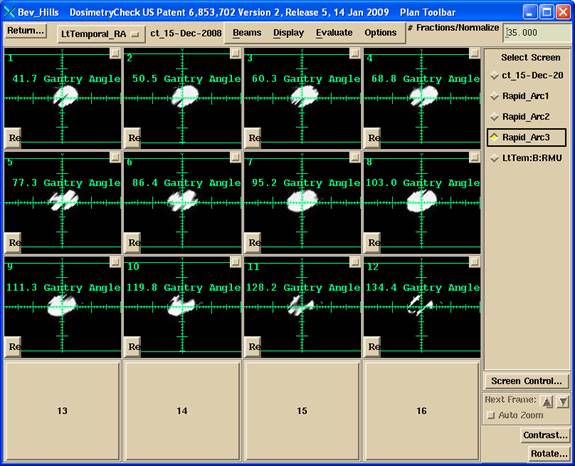
When you run Dosimetry Check, the fluence images for each beam will be displayed in a separate screen.

If you have to select the files for a beam manually, than under the Options pull down on the Beam Toolbar,

select “Read IMAT rmu files”. Select all the files for the beam. This operation will replace the prior list of files.