This manual is specific to the use of Dosimetry Check with the files exported from the TomoTherapy machine. This document covers the modifications for Dosimetry Check to work with the TomoTherapy machine. This manual is a supplement to the Dosmetry Check manual to cover the application of Dosimetry Check to support the TomoTherapy machine. Refer to the Dosimetry Check manual for the general operation of Dosmetry Check and the System 2100 manual for items not covered here.

The program uses the detector data file exported from the TomoTherapy radiation treatment system to reconstruct the patient dose distribution in the patient CT model from the detector file created during a treatment delivery without the patient present (pre-treatment) and during treatment (exit-transit). The program provides a feedback loop where the dose is reconstructed from measurement of the delivered treatment plan.

The purpose is to provide a final sanity check for the correctness of the delivered treatment plan.

The accuracy of the dose reconstruction is limited by the accuracy of the dose algorithm and the accuracy of measurement with the detectors. The user is advised to gain experience in the use of this method and the results obtained. Definitive criteria for plan delivery acceptance or rejection are difficult to define precisely. The transit dose reconstruction accuracy is further limited by patient positioning, changes in the patient anatomy, and limitations of the dose reconstruction algorithm. Experience will be needed to evaluate how this procedure should fit in with the institutions quality control policy.

Intended Use

Dosimetry Check is a standalone software product intended to be used by an experienced radiological physicist for quality control purposes only. Dosimetry Check is intended to check the correctness of x-ray treatment plans delivered from high energy charged-particle radiation therapy treatment machines by using a measurement of the applied radiation fields that are planned to be or have been applied to a patient, and computing the dose to the patient from the measured radiation fields. This product is to be used as a quality control check for the treatment planning system and delivery system.

Dosimetry Check quality control software uses the radiation fields that are measured with media such as x-ray film, electronic portal imaging devices (EPID), diode or ion chamber arrays, or in the case of TomoTherapy, a fan line detector array, and provides a theoretical calculation. Dosimetry Check computes the dose and dose distribution using the patient specific CT or other image set or alternately a phantom that is likewise scanned, to calculate the reconstructed dose that is then compared to the plan dose. The results reported can include the computed percent difference at specific point as compared to the patient specific radiation treatment plan.

Dosimetry Check does not provide any conclusions regarding the comparisons and does not provide any criteria to be used for interpreting the results. The experienced radiological physicist can reevaluate his patient specific radiation treatment plan in accordance with his clinical judgment.

This product is not a treatment planning system and is not to be used as one. This product only checks the applied dose based on the measurement of each x-ray field applied to the patient and provided in an exported file, and a theoretical calculation. This product does not provide any quality assurance that the fields are in fact correctly applied to and correctly aligned with the patient anatomy as planned. In addition, the product may be used to display the above dose on other fused image sets which could provide additional supportive quality information to the user regarding the correctness of treatment.

Disclaimers

This product is intended to be installed, used and operated only in accordance with the information within this manual, the Dosimetry Check and System 2100 manual for the purpose for which it was designed. Nothing stated in this manual reduces user’s professional responsibilities for sound judgment and best practice.

Users shall only install, use and operate the equipment in such ways that do not conflict with applicable laws or regulations which have the force of law. Use of the product for purposes other than those intended and expressly stated by the manufacturer, as well as incorrect use or operation, may relieve the manufacturer or his agent from all or some of the responsibility for resultant non-compliance, damage or injury.

Math Resolutions, LLC assumes no liability for use of this document if any unauthorized changes to the content or format have been made. Every care has been taken to ensure the accuracy of the information in this document. However, Math Resolutions, LLC assumes no responsibility or liability for errors, inaccuracies, or omissions that may appear in this document. Math Resolutions, LLC reserves the right to change the product without further notice to improve reliability, function or design. This manual is provided without warranty of any kind, implied or expressed, including, but not limited to, the implied warranties of merchantability and fitness for a particular purpose.

Users

This manual is written for trained radiation therapy physicist users of the Dosimetry Check product. Before attempting to work with this software product, read, understand, note and strictly observe all Warning notices, Cautions and Safety markings in this manual and messages presented to the user by the software.

Before attempting to work with this software product, make sure that this manual, the Dosimetry Check Manual and the System 2100 Manual and any Release Notes delivered with the software media pack have been thoroughly read and fully understood, paying particular attention to all:

Warnings
Cautions
Notes
Important Notices
User Notices

Training

Users of this product shall have received adequate training on its safe and effective use before attempting to work with it. Training requirements may vary from country to country. The user shall make sure that training is received in accordance with local laws or regulations that have the force of law. Information on training is available from Math Resolutions, LLC, or the distributor.

Location of Documentation

All applicable manuals are available on the Math Resolutions, LLC web site at the following link: http://mathresolutions.com/mancont.htm

These manuals may be downloaded and printed out if desired.

Hardware and Operating System Requirements

1. Hardware

For three dimensional surface shaded room view displays, an Open GL capable graphics card is required with 24 true color and a depth buffer. For added stereoscoptic three dimensional displays, an Nvidia Quadro fx card that supports stereo is needed with a single monitor capable of 120 Herz refresh rate, or the Planar Mirror System with two monitors. The program needs the same amount of memory and computation speed as a typical treatment planning system would need. For best operation, we suggest at least 4 gigabytes of memory. Because Dosimetry Check has to compute a beam beween every control point, we are recommending a 64 core computer so that the beams generated between control points can be computed in parallel to reduce the overall time required.

2. Operating System

The program will run on personal computers under the Linux or Windows operating system. The program has been tested under Microsoft Windows XP, Windows Vista, and Windows 7, and under Linux: Ubuntu 9.04. After installation, an install test is provided on the Math Resolutions website, www.MathResolutions.com, for the user or installer to follow for testing for the correct operation of the program on that particular computed and selected operating system. However, Math Resolutions, LLC, has tested the Dosmetry Check software on the operating systems identified above, if you use other operating systems that have not been tested by Math Resolutions, LLC, it is the user’s responsibility to validate the use of the alternate operating system with Dosimetry Check for your intended environment. The program is an X program using OSF/Motif and Open GL.

3. Third Party Software

The program is an X/Open Motif program using the specifications of the X window system version 11, OSF/Motif version 1.2 for the user interface, and Open GL release 1 for graphics. X, known as X11, originally developed at MIT Boston Mass. in 1987, is currently managed by the X Org Foundation (www.x.org). OSF/Motif is currently maintained by the X Org Foundation. To run on Microsoft Windows, the X server, Motif, and Open GL are required and are supplied by the software products Exceed, Exceed 3D, and the Motif dll out of Exceed XDK, from Open Text Inc., Waterloo Ontario Canada. Under the Linux operating system, X and Motif are native to Linux, and Open GL is readily available.

Installation Instructions

Installation instructions are provided on the Math Resolutions, LLC, website www.MathResolutions.com. The installer software is password protected. A license key is further needed from Math Resolutions to run the software. Contact support@MathResolutions.com for additional information.

Technical Description

Technical information specific to the use of Dosimetry Check with TomoTherapy is provided in this manual. Additional technical information regarding Dosimetry Check is available on the Math Resolutions, LLC website: www.mathresolutions.com

Warnings/Limitations of the Product

Warning: Cannot detect wrong field width.

Due to the Limitations of the TomoTherapy fan beam detector, Dosimetry Check cannot detect the wrong field width in the longitudinal direction.

The Tomotherapy detectors only measure a line through the center of the radiation field in the transverse plane. The field width in the longitudinal direction is reconstructed from a prior scan or computed from a source model fitted with the prior scan.

Wrong field width could result in an undetected large error.

The longitudinal field width is not directly verified and the dose shown to the patient will not accurately correspond to any error in the actual field width applied. An error in the applied field width could result in a large change in dose to the patient which will not be detected here.

The user is therefore advised to rely on some other method to verify the proper longitudinal field width.

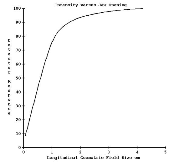
Only a line through the applied radiation field is being measured by the detectors. The jaw setting of the width of the field in the longitudinal direction is also read from the plan download and a prior measured profile is applied. If the wrong width were to be used, one would expect some change in the dose due to the increased radiation reaching the detectors for a larger width, or less radiation from a smaller width, as shown in the below graph. But the full affect would not be seen in the reconstructed dose since the wrong longitudinal profile would be applied. For example, if the plan called for the 2.5 cm field width but the 5.0 cm field width were applied instead, and the couch is indexing 2.5 cm for every gantry rotation, then each rotation would in fact be irradiating twice the volume. Which is to also say that the same volume would now be irradiated twice.

Hence the patient would effectively receive twice the prescribed dose.

The following table and graph shows data supplied by TomoTherapy. For a specified geometry jaw opening is a corresponding field width and radiation intensity, as shown in the below table:

Geometric Jaw Opening cm	Field Width cm	Intensity (normalized)
0.70	1.05	57.6%
2.0	2.5	93.6%
4.2	5.02	100%

From the above data, using a field width of 5.02 cm instead of 2.5 cm will result in a change of dose reconstructed by Dosimetry Check of 100/93.6 => 6.8% whereas the patient could well be getting twice the dose. The below curve gets flatter around the field width of 5.02 cm (geometric opening of 4.2 cm) and so large changes in dose to the patient due to a larger or smaller jaw opening from that field size would not register corresponding changes in the dose reconstructed by Dosimetry Check of the same magnitude.

Warning: Dynamic Jaw Position for TomoEdge is Not Verified.

TomoEdge has optional Dynamic Jaw capabilities at the beginning and end of the treatment with the effect of reducing the penumbra at each end of the treatment in the inferior and superior directions. The user can choose Fixed or Dynamic treatment modes. Dynamic is only available on the 2.5 and 5.0cm jaw widths, not the 1cm width, according to our understanding. Because the detector only measures a line through the radiation field in the transverse plane, the use of dynamic jaws cannot be detected nor the position of the jaws determined during treatment or verified from the detector reading alone. Prior to version 4 release 9 of Dosimetry Check, the applied radiation fields were reconstructed in Dosimetry Check from the detector readings assuming a constant jaw opening along the long axis of the machine, and consequently the dose could not be properly reconstructed in the regions of the dynamic jaw movement. We have presently no way to verify the jaw position (see warnings above) since the detector only measures on the central axis.

Accounting for TomoEdge in DosimetryCheck

With Version 4 release 9, however, by fitting a source model for the longitudinal direction, some account can be made for the asymmetric jaw openings using the jaw positions from the plan. Version 3 release 0 or later of ReadDicomCheck must be used to produce a control points file with the jaw positions for Dosimetry Check to read during dose reconstruction.

Source Model

Since there is no flattening filter, only a one part source model is needed. And since the profile need be computed in only the longitudinal direction, the source model can be one dimensional. The source intensity is represented by an exponential I( r ) = B/2 exp(-Br) where B is a fitted paramenter and r the distance from the central ray. Given a point in space, the area under the curve is computed for the length of the source model the point is exposed to through the opening in the jaws. Added to that is the rest of the source attenuated by a factor T, which is another fitted parameter. Lastly, if the point is under a jaw, the sum of the two prior components is multiplied by another exponential exp(-At dist) where At is a fitted parameter and dist is the distance the point is from the jaw edge (computed at distance 85 cm). This last term corrects for increased attenuation at increasing slant distances. A nominal distance from the source to the jaw is defined. The Parameter B will basically scale if this distance were to be changed, and so is not a fitted parameter.

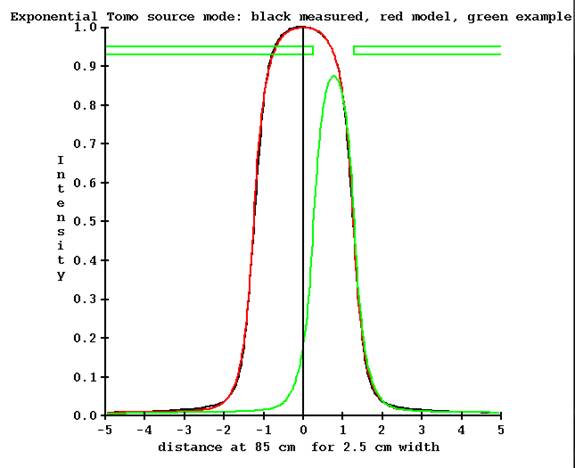
Program FitTomoSourceModel will fit the source model for all three nominal widths of 1.0, 2.5, and 5.0 cm. Program FitTomoKernel will also fit the source model for the chosen width. The source model parameters will be written to the file TomoSourceModelFitnn.txt where nn is the nominal width in mm, in the X06 directory of the machine directory. A plot file is also produced as shown below (plot drawn by program DrawGraph).

Shown in the below figure is the computed profile from the fitted source model in red, and black the measured profile, for the 2.5 cm jaw width. In green is shown the profile for the starting jaw position at the start of TomoEdge. The jaws are at 0.253 cm and 1.279 cm at 85 cm respectively for the inferior and superior jaw (Y machine axis in beam’s eye view coordinates). The ending of the treatment is reversed (-1.279 and -0.253 cm). Note that the detector is on the central axis where the profile has a value of 0.192 relative to 1.0 for the symmetric nominal opening.

Detector is out side of the beam for some jaw positions.

Hence the detector is basically outside of the field. We can estimate the intensity profile by multiplying this curve by the factor of the detector reading divided by the value of 0.192 on the central axis where the detector measures. Using an off axis measurement at this point to measure the beam introduces some uncertainty in the result.

The situation is worst for the nominal 5 cm jaw width at the start and end of TomoEdge treatment:

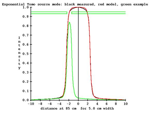
The jaw position is shown at the end of the treatment with the jaws at -2.370340 cm and -1.375920 respectively (at 85 cm). The measurement point on the central axis is completely outside of the beam, with a value of 0.024 relative to 1.0 for the nominal jaw opening. To estimate the intensity profile will require multiplying the profile by the detector measurement made outside of the beam (on the central axis), which will be a small number, and dividing by the computed model value of 0.024. This clearly can introduce large uncertainties.

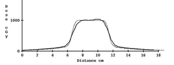
For the 2.5 cm nominal opening, using the computed profile estimate gave reasonable results. Shown below is the profile for a plan done in the Cheese phantom without correcting for tomo edge and with correction:

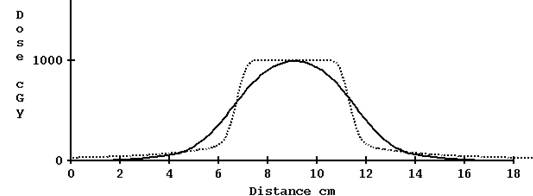
Computed profile not corrected for TomoEdge solid versus plan dotted, 2.5 cm width

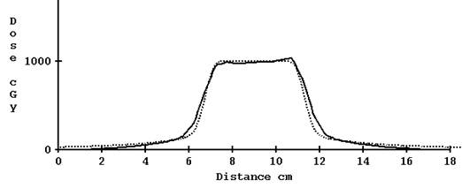
Computed profile corrected for TomoEdge solid versus plan dotted, 2.5 cm width.

Problem with 5 cm width TomoEdge

For 5 cm width, however, the results are not so good with the correction for TomoEdge:

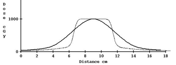
Computed profile not corrected for TomoEdge solid versus plan dotted, 5.0 cm

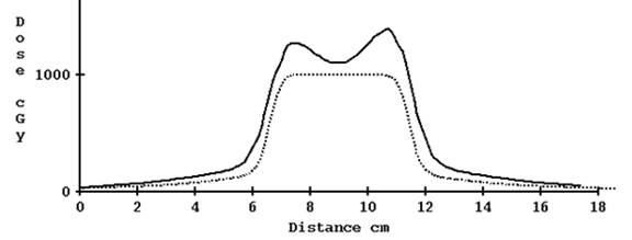
Computed profile corrected for TomoEdge solid versus plan dotted, 5.0 cm

Compromise for source model applied to jaw width 5 cm

We wish to keep the system dependent upon measurement by the detectors and not to rely on actual leaf opening, as we are already relying on the stated jaw position for the plan. A compromise was arrived at to limit the denominator in the normalization ratio to a minimum value. A default value of 0.15 was arrived at by trial and error giving the result shown below:

Computed profile corrected for TomoEdge solid versus plan dotted, 5.0 cm with compromise limiting the denominator of the normalization factor.

In effect, the more extreme asymmetric jaw openings are not fully accounted for, resulting in the penumbra created by the dynamic jaw movement not being as accurately reconstructed. We can accept some small error here compared to the example shown below of not accounting for the created penumbra at all, as the main interest is in the interior of the actual treatment area between the penumbra areas, as shown in the below example case image:

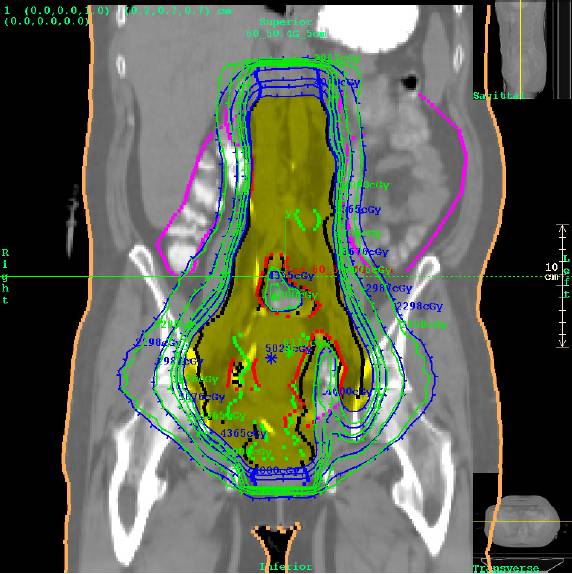
Dose comparison for a case where the dynamic TomoEdge movement is not accounted for at the ends of the treatment. Even in this worst case, the treatment in the area of interest is verified. Planning system isodose in green, Dosimetry Check in blue. See below for example of TomoEdge accounted for.

2.5 cm prostate case with TomoEdge accounted for:

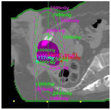
Prostate case with TomoEdge with dynamic movement accounted for.

Plot along machine Y axis (axis of rotation, feet to head) for the above case:

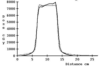
File controlling the limit value:

The default limiting value is 0.0 for 1.0 and 2.5 cm jaw widths, and 0.15 for 5 cm width. The value may be changed with the file TomoSourceModelLimit50.txt (50 for 50 mm width, use 25 for 25mm width should there be a reason be to apply the limit there also):

/* file format version */ 1

// Minimum number to divide the profile by for asymmetric jaw

0.15

in the machine’s directory in the energy sub-directory X06.

Warning: Gantry angle and couch position not tested.

This method does not test that the radiation is applied correctly to the patient anatomy.

The coordinates to apply the measured radiation fields to the patient are read from the Dicom RT plan download. Therefore it is assumed that the radiation fields are being applied to the correct place on the patient. The gantry rotation is assumed to be correct and the couch indexing is assumed to be correct.

Warning: Keep Final Calibration:

Be aware that running either FitTomoKernel, ComputeCalConstant, or SetTomoDetectorCalibration will replace the dose convert constant with that computed from the specification in the below TomoCalibration file.

Warning: If couch is in, you must use the same couch height for all pre-treatment clinical case runs.

The couch correction that is applied at each detector is the ratio of the detector measured with the couch in to the couch out at a particular gantry angle. The couch must be at the same height for the measured ratio to be correctly applied.

Error and Alarm Messages

Error messages are presented to the user in a pop up window and are written to standard out (C language printf and cout statements). Standard out is redirected to the text log file dcstdout.log when Dosimetry Check is run from the DosimetryCheckTasks executible. Otherwise, if run from a command prompt window, standard out is to the command prompt window. These messages will result from conditions where the program is unable to complete a function, such as not being able to read a selected file.

The following is a list of pop up messages added for the support of the TomoTherapy machine:

1. Before clearance:

Support for TomoTherapy has not yet been cleared by the US FDA for distribution in the US, nor by the European body for CE Mark.

2. If you do not have a license to use the TomoTherapy feature of Dosimetry Check and a TomoTherapy machine has been selected for a beam:

Support for TomoTherapy is not available. Program will not compute dose.

3. If you did not pick a TomoTherapy machine in one of the TomoTherapy specific utility programs that is a windows program:

Pick a TomoTherapy machine.

4. If you are doing pre-treatment and you have a couch correction file:

Pretreatment detectors will be corrected for couch height of: (with the couch height displayed)

5. If you are doing pre-treatment and do not have a couch correction file:

Pretreatment must have been done with couch out of the beam. Otherwise create a pretreatment couch correction file.

6. If you create a beam in Dosimetry Check and select a TomoTherapy machine:

TomoTherapy width to use is not specified yet. You have to read in a plan first.

7. If the file size of the selected detector file is too small:

There are not enough detector rows for the number of control points.

There must be at least number of control points less one reads of the detectors.

Did you select the correct sinogram detector file?

8. If the detector file you selected is not the expected size.

The file size was not correct for the number of rows expected.

See log file for this program after exiting.

9. If you did not select a couch in and a couch out detector file in the couch correction utility:

You have not read in both a couch in detector file and a couch out detector file.

10. If you are attempting to compute the dose but have not selected a detector file.

No needed detector data files for TomoTherapy

11. Working message while processing the detector file to create the TomoTherapy radiation fields.

Generating Tomo Fields

System Description

Dosimety Check is a software program that will compute the dose and dose distribution to the patient from a measurement of the radiation fields that are applied to the patient. The dose so computed serves as a means to verify the correctness of the radiation treatment and to serve as a final sanity check. The radiation fields are measured with media such as x-ray film or electronic devices that will measure over the area of the field, such as electronic portal imaging devices (EPID), or diode or ion chamber arrays.

System2100 serves as a foundation that provides basic image display functionality for Dosimetry Check, a contouring package, and other useful functions such as image fusion.

To extend Dosmetry Check to support the TomoTherapy machine, the device uses the data measured by the fan beam radiation detector that is part of the TomoTherapy machine. The detectors capture the radiation intensity periodically at predetermined gantry angles and couch positions, known as control points, from the treatment plan. The detector only measures the intensity across the center of the radiation beam in the transverse plane. A prior measured profile in the perpendicular longitudinal direction is then applied to complete the radiation field map. The radiation field map is then applied as a stationary beam at the center gantry angle and couch position for the integration period (between two control points), from which the dose to the patient is computed. The patient dose is then summed up from all such radiation field maps.

Measured Parameters

The measured parameter is the detector file measured by and exported from the TomoTherapy machine. Additional data for the geometry of the machine and detector and for generating the pencil beam dose kernel are provided in the Theory of Operation section of this manual.

Accessories

There are no accessories sold with this software product or its included utility program for supporting TomoTherapy, or accessories authorized to be used with this product with the exception of the hardware/operating system requirement.

Start Up/Shut Down Procedure

Run the utility program DosimetryCheckTasks from the desktop icon, from the start menu, or from a command prompt window. Then select the program ReadDicomCheck (“Read in Dicom RT protocol files”) to import a plan from the planning system by selecting the Dicom RT exported from the planning system. Run the Dosimetry Check execitible by selecting “Run Dosimetry Check program.” When run from DosimetryCheckTasks, standard out is piped to a text log file in the home directory. Additional information is written to standard out during program execution.

The Dosimetry Check executable (any of the executables) may also be run directly from the command prompt window from the directory that it is installed in, by default c:\mathresolutions, unless installed elsewhere. Standard out will be written to the command prompt window unless you add the argument –s, which will redirect it to a log file.

[For pre-clearance beta sites, the Dosimetry Check executable must be run from the command prompt window by running DosimetryCheckTomo.exe or on a 64 bit platform DosimetryCheckTomo64.exe.]

To exit, hit the exit button on the left on the main tool bar. You must take this normal exit for the program to remove a lock file on the patient’s data directory. The lock file prevents concurrently running Dosimetry Check executables from accessing the same patient records.

Security

Access to the computer and directories where data are stored and used by the Dosimetry Check program is the responsibility of the user.

IEC 60601-1 Medical electrical equipment

Part 1: General requirements for basic safety and essential performance

IEC 60601-1 is not applicable to System 2100, or Dosimetry Check since these products are software.

Assumptions

The user must be aware of what is not checked. The patient is assumed to be in the correction position for treatment. It is assumed that the gantry rotates correctly and that the couch indexes correctly. The model of the patient from the snap shot of the planning CT scans used here is assumed to represent the patient. The exit-transit reconstruction algorithm ignores scatter from the patient to the detectors (there is an air gap and the field is narrow, limiting scatter). Any point spread in the detectors are also ignored. Finally, the program cannot verify the field width in the longitudinal direction (see warning above)..

Theory of Operation

1. Pre-treatment quality check

For the pre-treatment quality check, the treatment is performed as if the patient were there. But the couch is withdrawn from the tunnel so that it is not in the beam, or if it cannot be withdrawn, the couch can be in the beam but without the patient. If the couch is in the beam, the couch must be at a consistent height so that a pre-measured couch correction file for the detectors can be used as described below.

The fan line detector that is part of the TomoTherapy machine measures the radiation emitted during the dry run without the patient. It should be noted that this record does not include the couch position, the gantry angle, or the field width (along the long axis of the couch and patient) and the detectors only measure a line through the center of the radiation field in the transverse plane. The detectors integrate the radiation field between control points. If there are N control points, there will be N – 1 measurements of the detectors. Each measurement of the detectors results in a row of floating point numbers, one for each detector. The collection of all the N- 1 measurements will be referred to here as a detector sinogram file or simply as a detector file. There may be additional rows of data in the exported file from warm up of the machine when the leaves are all closed. It is assumed that the last N-1 rows are for the N control points. A control point consists of a couch and gantry angle coordinate specification, and a list of the leaves that are open at that point.

Prior to Version 4 Release 9, the pre-measured longitudinal profile of the beam is applied to each detector, normalized by the reading from that detector, to form a two dimensional x-ray intensity map of the radiation field in a plane perpendicular to the central axis. With release 9 a source model computes the longitudinal profile taking into account the position of the jaws in that direction. This radiation field map provides the intensity value for each ray in the radiation beam over the area of the beam. The intensity map will reflect the result of which leaves were open and of the output of the radiation source during the integration period. With TomoEdge, a compromise in normalizing the longitudinal profile was necessary as some of the beams are entirely off axis with the detector outside of the beam. See “Source Model” above.

A stationary beam is then modeled from this intensity map, at the gantry angle and couch location at the center of the integration period (the average of coordinates between the two control points) and used to compute the dose to the patient with an external beam dose algorithm. The dose to the patient is computed from the sum of all such beams. If there are N control points, there will be N-1 beams. The continuous movement of the couch and gantry is approximated by the N-1 fixed beams.

2. Transit quality check

For transit dose reconstruction that is performed using the detector file exported from the TomoTherapy machine, the detector file records the radiation reaching the detector during treatment of the patient. The method used by Dosimetry Check is to compute the water equivalent path through the patient (and couch) to each detector, and divide the detector reading by the attenuation computed for that path. There is no correction for any scatter reaching the detector. Due to the air gap and small field widths in the TomoTherapy machine scatter can be ignored but that will limit the accuracy attainable.

Before computing the dose, preferably before selecting the detector sinogram file, all issues of CT number to density conversion, couch modeling, patient outline, any assigned densities to region of interest (ROI) volumes, for a final patient model must be complete before converting the exit detector readings to pre-treatment readings. Then from that point, the dose computation proceeds as it does for pre-treatment.

TomoDirect

A single detector file may be read for TomoDirect cases. The single file will contain the detector readings for all the treated beams. Currently, there is nothing in the file that indicates the order in which the beams were treated. The program assumes that the beams are treated in the order of gantry angle: 180 to 270 to 359 to 0 to 179, where the gantry is at a fixed angle for each beam. If this order is not followed, the program will be assigning the wrong detector record to each beam.

Upon selecting the detector record file, the program will pop up a tool for the user to review and select the order in which the beams were delivered, as shown below:

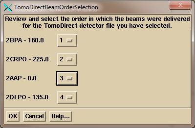
The name of each beam is shown with the beam gantry angle. To the right of the beam name – angle is an option menu. And option menu is a pull down menu that shows the current choice. If the beam order needs to be change, select the order number for each beam using the option menu choices, which will the number 1 through the number of beams:

Because the beam order has been demonstrated not to be fixed, AutoRunDC will not support TomoDirect.

Given the number of control points for each beam, the program will attempt to find the corresponding detector record. If there are N control points, there will be N – 1 integrations. The program will expect to find beam on intensity after the first control point integration and for the last integration between the last two control points, and no beam on intensity before the first integration and after the last. If this condition is not met, the program will flag an error and not import the detector readings.

Select the TomoDirect file from the plan toolbar only.

Warning: Do NOT select the detector record file from the beam toolbar for TomoDirect.

When a detector file is selected from the beam toolbar, the program assumes that the detector record is for that beam only and uses the last N – 1 rows (integrations) in the file assuming that the record ends at the last control point. Everything preceding is ignored. So if there are four beams in the detector record file, beams 1, 2, 3, and 4, and the file is selected for beams 1, 2, and 3, those three beams will incorrectly use the last detector record for beam 4. If the program detects that the detector file is larger than it should be, it will flag a warning, but such detection cannot be assured.

Requirements for User Prior to Use (Commissioning)

All of the following must be accomplished before you can begin using Dosimetry Check with a TomoTherapy machine.

1. Geometry File

The geometry of the detector must be described to the program. This is accomplished in the Geometry File as described below in the beam data requirements section.

2. Beam data

The beam data between machines is probably close enough that the generic data supplied from a single machine need not be replaced. However, you may want to check the percent depth dose in the files starting with the letters “CA” against your own data to make that decision. Compare the same for the lateral and longitudinal profiles which were measured in water. If your data is different, then read the beam data requirements below and replace the data.

3. CT number to density curve

You will need to entire into Dosimetry Check a curve for CT number to density. See the section on this in the Dosimetry Check manual. While all CT scanners generally operate at 120 kVp, we find a wide variation in the data used for this purpose at different sites. The curve should be generated from biological equivalent materials.

4. Density of Phantom Used for Calibration and Testing

You should measure the water equivalent of the density of the phantom that you use for the absolute calibration of the detectors. You cannot depend upon your CT number to density curve to give you the water equivalency of any phantom, which, hopefully, was generated from biological equivalent materials. Beam data is measured in water. Mono-energetic dose kernels were computed for water. Thus for any material, a water equivalent density is needed. This should be measured for the same beam or nearly the same beam energy. What matters is NOT the physical density in gm/cc or the electron density relative to water (although that tells us something). The processes involved are photo-electric effect, Compton scatter, and pair production, which depend upon things like atomic number, electron density, and the x-ray energy. So let us simply measure with the megavoltage beam in question what the material does compared to what water does.

We can suggest two methods to do this:

a) Transmission measurement

Set any field size and fix an ion chamber with build up cap some distance below the material. First make a measurement with only the support system there, then put the phantom there and make a measurement. The ratio is the attenuation.

Then remove the phantom and make a measurement with water (in hopefully something with a thin bottom or near water equivalent material, or make the first measurement with an empty tank. Make the above measurements by putting the phantom in the same empty tank). Make measurements for more than one water thickness so that the attenuation measured will bracket that measured for the phantom. For example, if the attenuation for 30 cm of the material was 0.23 and you measure for 30 cm of water 0.21 and for 32 cm of water 0.24, then one can interpolate the water equivalent of the phantom material:

>tools.dir\Interpolate.exe

enter x1 y1 x2 y2 x

0.21 30 0.24 32 0.23

result: 31.333334

and the material looks like 31.33 cm of water, or the water equivalent density is 31.33/30.0 = 1.044

Will the result change with the field size you use? Probably not or only slightly. Both the material and the water will contribute scatter to the ion chamber, but the amount of scatter can be expected to be nearly the same for a nearly water density material. An air gap between the material and the chamber will reduce the affect of scatter, as will a small field size. For transit, Dosimetry Check has to compute the attenuation of rays through the patient, so the above determines equivalency the same way the data will be used. Once you have the water equivalent density of the material, you can contour the material as a region of interest volume (ROI) and assign that density in Dosimetry Check (see Outlining Regions of Interest in the System 2100 manual and Stacked Image Set: Density in the Dosimetry Check manual).

b) Depth dose measurement

Place the ion chamber in the material at some depth and make a measurement.
Then put the ion chamber in water. Keep the distance to the ion chamber the same but vary the depth of water until you get the same reading (or interpolate between two bracketing readings). Take the ratio of depths for the water equivalent density.

Will method (2) agree with method (1)? We would not expect much of a difference.
You can always study this and publish you results.

5. Detector calibration

Your detector array will have to be calibrated for each of the nominal field widths (in the longitudinal direction). First you will have to do the relative calibration as describe below. This will involve running the machine with all leaves open while collecting detector data.

Then an absolute calibration of the detectors is required. You will have to create a plan for a phantom where you can measure the dose that is actually delivered. You will adjust a value in a file, as described below for absolute calibration, to normalize the dose computed by Dosimetry Check to agree with the measured dose.

6. Couch for pre-treatment runs

For all pre-treatment runs, the couch is to be out of the beam. If the operating system of your machine does not allow you to do this, then you will first have to generate a detector couch correction file as described below.

7. Detector transit correction

A number of different model detectors have gone into the TomoTherapy systems. Some detectors have a large energy dependence and will not accurately measure the transmission through water. This must be corrected for to be able to do transit dosimetry with Dosimetry Check. See the section below on water transmission measurements with the detectors to create the correction file.

Patient treatment quality check work flow with Dosimetry Check

1. Dosimetry Check application

Automation

If you have the version of the TomoTherapy operating system that will export the detector file in a Dicom format file, then you have the option of using the automated system provided by AutoRunDC. To do so, you export the Dicom detector file to either the pre-treatment folder specified by file EPIDImagesDirectory.loc or to the exit folder. As only the patient name is in the Dicom file, the automation program can only assume the latest plan downloaded for the patient is to be used. See the AutomatedDosimetryCheck manual on how to set up the EPIDImagesDirectory.loc file (and note that you will never use the calibration folder). You must have first imported the plan and set up the external outline, the couch model, and made selections for the auto report (see below).

Manual

If you can only obtain the binary file for the detector, the you will have to run the Dosimetry Check executable. Select patient, select plan, and then select the detector file to read it in as described below.

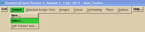
The Dosimetry Check main module pushes the System 2100 main toolbar. Functions specific to DosimetryCheck are under the Plans pull down on the main toolbar. See the Dosimetry Check manual for details.

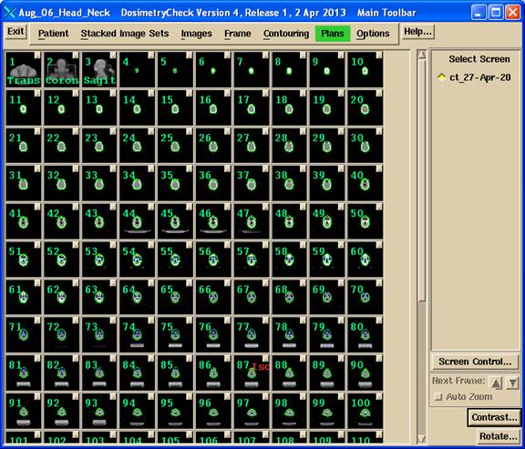
Dosimetry Check main window

An example of the main application window is shown below with the Main Toolbar active. The currently selected patient’s name is shown on the left of the title bar on the main window, “Aug_06_Head_Neck”, in the example below. Next on the title bar follows the name of the application, then the version of the application including the assigned date of the release, followed by the name of the current toolbar that is displayed.

Toolbar Organization

The toolbar organizational diagram for Dosimetry Check is as follows.

2. Dicom RT plan download

Down load the plan from the TomoTherapy planning system in Dicom RT format. Run program ReadDicomCheck (see above Start Up and see the Dosimetry Check manual section on Dicom RT download). Create your patient entry if the patient is not already in the Dosimetry Check system. The patient entry is a directory (folder) name in the directory designated for patient data (file PatientDirectory.loc in the program resources directory, rl.dir by default, see Program Resource files in the System 2100 manual and Files in the Dosimetry Check manual). You can use the Auto Read function of that program (see the documentation for this program in the Dosimety Check manual). You want to read in the patient CT scans, the structures file, the plan file, and the 3D plan dose file. In Dosimetry Check, an isocenter point will be reported as the center of the couch position between the first and last control points.

3. External outline

In Dosimetry Check you will also have to create an external body outline if one is not downloaded from the planning system. See the outlining tools in the System 2100 manual for the auto body outlining tool. You can do this function in the ReadDicomCheck executible or the Dosimetry Check executable. The ROI must be selected as the external outline.

4. Couch dose correction

If you want to correct for the TomoTherapy couch for dose computation, you will have to create a region of interest (ROI) structure for that. This is easily done by outlining the couch on the first and last CT scan. Outlines in parallel planes are connected and shape interpolation is performed by default in between the outlined slices. [You can outline in other parallel planes besides transverse planes, see the contouring, outlining, tools in the System2100 manual.] See the “Couch Correction For Dose Calculation” section below. Contouring is accessible in the ReadDicomCheck executible or the Dosimetry Check executable.

5. Pre-treatment quality check

Retract the couch, and run the treatment without the patient being there. You must then export the file written by the TomoTherapy detectors from the dry run.

It is preferred that the couch not be in the beam for a pre-treatment dry run. However, if you cannot extract the couch for the dry run without the patient, there is an alternate work around described below that enables a correction to the detector readings.

Detector integration is generated during the delivery of the treatment run, resulting in a detector file.

6. Transit treatment quality Check

Detector integration is to be generated during the treatment of the patient, resulting in a detector file. All issues regarding the patient model must be resolved before computing the dose, including the generation and selection of the external patient outline. For best results the couch should be corrected for. See the below section on “Couch Correction for Dose Computation”. When the patient model is complete, select the detector file taken during treatment as described below.

7. Run Dosimetry Check

Run Dosimetry Check. On the Main Toolbar select the patient

and then select the plan that was created when you imported the plan above in ReadDicomCheck.

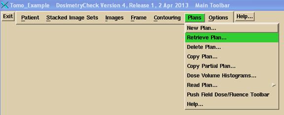
If there is only one plan under the patient name, it will be selected and read automatically. If there is more than one plan, you will be presented a list to select from.

The Plan toolbar will be pushed. If there is only one beam and it is a TomoTherapy beam, you may select the sonogram from the Beams pull down on the plan toolbar:

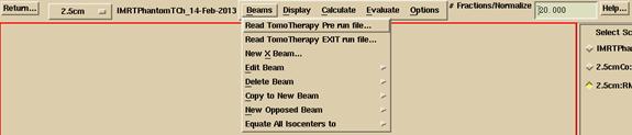
You must select the correct button to read in a pre-treatment detector file or an exit file. It is only here with your choice that the program can distinguish between the two measurements. If you were to select a transit run file for a pre-treatment run, you will get very small doses computed. If you select a pre-treatment run file for a transit file, you will get very large doses, in both cases by a factor of around five for a 30 cm thick body.

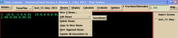
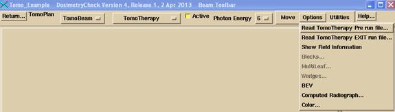
Otherwise on the Beams pull down menu on the Plan toolbar, select the TomoTherapy beam to be edited. The Beam toolbar will be pushed. Under the Options pull down, select to read in the detector file measured above and exported. For pre-treatment cases, use the first choice on the Options pull down show below and select the pre-treatment detector file. For transit dosimetry, select the second option on the Options pull down and select the detector file measured during treatment (an exit detector file).

Your selection is the only way the program can distinguish between a pre-treatment and exit detector file. Note that the detector file just consists of rows of floating point numbers, one number for each detector, one row for each integration.

Then hit the return button on the Beam toolbar to return to the plan toolbar. You are ready to evaluate the plan.

8. Comparison of Dose

See the Plan section of the Dosimtry Check manual on how to make dose comparisons using the comparison tools provided to compare the dose reconstructed by Dosimetry Check for the pre-treatment or exit-transit to the planning system dose.

Dose Computation

You have an option to simulate the plan with a beam between each control point, or to combine every two control points, in the latter case reducing the number of beams to be computed by a factor of two. For example, control points 1 and 2 would be combined, and then control points 3 and 4. With this reduction, there would be a beam every 14 degrees instead of every 7 degrees (the control points being 7 degrees apart). With this latter chose, a fluence is still generated between each successive control points taking into account the possible presence of the couch at the particular gantry angle and the transient correction made for exit-transit dosimetry. But the two fluences are then added together and applied at the average gantry and couch position. The choice is made in a program resource file TomoPreferences.txt and an example file follows:

/* file format version */ 1

// Enter 1 to compute each Tomo control point.

// Enter 2 to combine every two Tomo control points.

There will be some small lose of accuracy in making this approximation, but the compute time will be halved. For version 5 and after, you have the choice of pencil beam or convolution/superposition “collapsed cone” dose algorithms. See the Plan Toolbar in the plan section of the main Dosimetry Check manual, under Calculate.

9. Couch Correction for Dose Computation

For pre-treatment, the computed dose will decrease as the couch density increases.

For transit, the computed dose will increase as the couch density increases. The latter effect is because the program first converts the exit detector signal by dividing the exit signal value by the attenuation computed along the ray from the source of x-rays to the detector, to produce the detector signal as if the patient were not there. So while increased couch density will decrease the dose to the patient from rays from below that go through the couch, the fluence will have first been increased by rays from below and above that go through the couch.

The couch correction for pre-treatment detector files that were measured with the couch in the beam is not a dose computation matter here and is a separate issue describe later below.

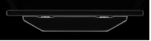
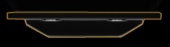
10. Outlining the Couch

The TomoTherapy planning system can burn the treatment couch into the CT scans and export the CT scans. It is only necessary to outline the couch on two end CT scans (the superior most and inferior most CT scan) to create the couch model. When contours overlap for two successive contours in parallel plans, the program will connect the contours (shape interpolation is done in between but that would not be much of an issue here with a contour that is not changing). See “Outlining Regions of Interest” in the System2100 manual.

Adjust the contrast so that all of the couch can be seen. See “Main Screen” in the System2100 manual. Simply slide the contrast width to the left on the contrast control.

After contrast is set:

Then from the main toolbar, select Contouring. Create a couch ROI, and select “Auto Frame Contouring” for the method. Click the mouse on a space right above the couch boundary and then on the boundary (use the upper edge). Selecting the correct two points will result in a complete contour. If not, then use Mouse contouring to contour the couch. With mouse contouring, you can select to project the next nearest contour in a parallel plane and to use and accept that contour.

Contoured couch:

The program will compute a 3D model from the two end contours, shown below in a 3D perspective room view:

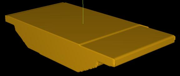
For the version of Dosimetry Check after June 2012, the couch will be considered in calculation and you do not have to create a combined body – couch volume as described below.

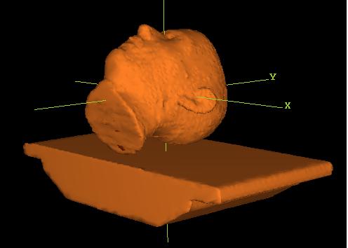
But for earlier versions, you must combine the external outline ROI and the couch ROI. See the section “New Volume from Other Volumes” in “Outlining Regions of Interest” in the System2100 manual. Then select this ROI as the patient model. See “Stacked Image Set: skin, density”, in the Dosimetry Check manual. Shown below is a combined patient couch model in a 3D perspective room view:

11. Couch Density

a) Use CT number conversion

One should use a phantom with biological equivalent inserts to run a CT number to density curve for dose calculation. See “Stacked Image Set: skin, density”, in the Dosimetry Check manual for details. Such a conversion is for biological materials. The couch top is most likely not water or biologically equivalent. Therefore the mapping of CT numbers to density might not be very accurate. However, the CT number to density mapping might be accurate enough for the computation of dose and for converting transit detector files to pre-treatment.

b) Set Couch Density

If not, instead consider measuring the water equivalence of the couch top. To do this, measure the transmission through the couch with the TomoTherapy beam and an ion chamber. Make similar transmission measurements through water with a measurement bracketing the couch measurement and compute the amount of water that results in the same attenuation. A measurement on a TomoTherapy couch 8.5 cm thick resulted in a value of 2.0 water equivalency for a water equivalent density of 2/8.5 = 0.2353. Set the couch ROI density to the value obtained. See “Stacked Image Set: skin, density”, in the Dosimetry Check manual. Be sure to set the density for the ROI couch volume, NOT the combined couch patient ROI volume. In ray tracing through the patient volume, the program will use the assigned density for points inside the couch ROI volume. See also in water transmission measurements below.

Beam Data Requirements

Some beam data is needed for Dosimetry Check to be able to reconstruct the dose from the detector file. The required information is described below. However, generic data supplied is most likely to be accurate enough for dose reconstructions purposes. The exception will be the Geometry file described below which must describe the detector in the particular TomoTherapy machine.

a) Geometry File

The Geometry file describes the TomoTherapy unit to Dosimetry Check. The file follows the text file standard for System 2100 (the underlying software on which Dosimetry Check is built). The file is self documenting and an example file follows. Note the field widths are nominal widths. The file should be changed to correspond to the detector array that is in the machine.

/* file format version: */ 3

/* type of machine 1 gantry, 2 TomoTherapy */ 2

/* Source Axis Distance (cm) = */ 85.00

/* Positive gantry rotation: +1 = clockwise, -1 = counter-clockwise */

/* angle when pointed at the floor */ 0

/* Y axis, positive couch longitudinal direction, positive is +y IEC. Enter -1 here if couch longitudinal is positive in, otherwise 1. when moves toward gantry) */ -1

/* center position value (cm) */ 0.00

/* number of widths */ 3

// nominal widths cm

1.0 2.5 5.0

/* number of channels: */ 643

/* number of detectors */ 640

// counting detectors from zero:

/* Detector zero connects to channel */ 0

/* channel number for dose monitor */ 640

/* radius of detector cm */ 98.6

/* isocenter to detector distance cm */ 47.3

/* spacing of detectors along arc cm */ 0.118

/* nominal center index counting from zero */ 319.5

/* c.a. in index coordinates relative to center */ 0

/* First detector on left 1, or on right -1*/ -1

// below two entries are used for the water transmission utility:

/* number of leafs */ 64

/* leaf width at isocenter cm */ 0.65

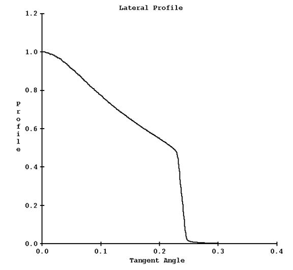
b) Lateral Profile File

The lateral profile should be measured in air, but an in water measurement at dmax will also suffice. This file has the same format as the InAirOCR file as it serves the same purpose, but has the name LateralProfilenn.txt where nn is the field with in mm such as LateralProfile25.txt. Here this profile describes the open beam across the treatment couch with the leaves wide open for the set field width. This file is used to calibrate the detectors on a relative basis to each other. The format is as follows:

/* file type: 8 = In Air OCR or Tomo lateral */ 8

/* file format version: */ 1

/* machine directory name: */ <*TomoTherapy*>

/* energy = */ 6

/* date of data: */ <*23-Dec-2010-10:14:44(hr:min:sec)*>

/* Number of data pairs: */ 516

// Must be in increasing order, starting with central axis

// Tangent OCR

0.000000 1.000000

0.000215 1.000000

0.000867 1.000093

. . .

0.296643 0.003195

0.297725 0.003148

0.298918 0.003105

If a profile is measured, both sides should be averaged for this file. Notice that the displacement is the tangent a ray makes with the central axis.

A plot of this curve is shown below for the field width of 25 mm:

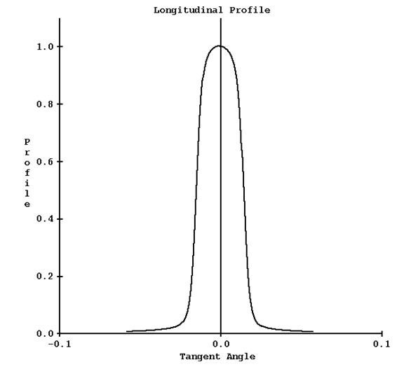
c) Longitudinal Profile File

As the lateral profile, this profile should be measured in air, but a scan at dmax depth will be close enough. The format is different from the lateral profile in that both sides of the profile is saved rather than averaged. The file name is LongitudinalProfilenn.txt where nn is the field width in mm as in LongitudinalProfile25.txt. This profile is used to define the field shape perpendicular to the lateral profile, along the long axis of the couch. The profile is to be measured with the leaves wide open for the set field width. As the detectors only measure the x-ray intensity on a single line in the lateral direction, this profile is necessary to define the shape of the field in the longitudinal direction for the stated field width. An example file follows:

/* file type TomoTherapy longitudinal */ 2

/* file format version */ 1

/* energy */ 6

/* slice width setting cm */ 2.5

/* number of data pairs */ 281

// tangent value

0.057440 0.007245

0.057008 0.007290

0.056573 0.007543

. . .

0.000613 0.999262

0.000180 1.000000

-0.000254 1.000872

-0.000652 1.001200

. . .

-0.057949 0.008311

-0.058382 0.008221

-0.058816 0.008176

A plot of this curve is shown below (for 25 mm width field):

d) Depth Dose Profiles

A correction table is computed for points off the central axis from in water scans for the leaves wide open, to correct for change in penetration (effective energy). The file that holds the input data for this correction has the same format as the in water diagonal scans for gantry mounted treatment machines, except that here the profiles are measured in the lateral plane of the central axis. Depths scanned in water should be 1.5, 5, 10, 15, and 20 cm, and deeper if possible. The file name is DiagFanLinenn.n_w00_06 where nn.n is the field width in cm, such as DiagFanLine02.5_w00_06 for 2.5 cm. A utility program is available to read in water scan profiles and write this file out in the expected format. See Beam Data for Dosimetry Check.

e) Central Axis Depth Dose

The central axis depth dose for the leaves wide open for the field width is store in a central axis file. For nominal purposes, the width of the field in the lateral direction will be designated at 50.0 cm in the file name convention. The second dimension will be the width of the field in the longitudinal direction. A file for each width is stored in the file CAFileListw00_06 where the gantry mounted file name convention continues to be used. The file for 2.5 cm width has the name CA50.0x2.5_w00_06. See the Dosimetry Check manual for the file format. From the single scan for each width, a spectrum is fitted for the width. The depth dose data should start at 0 depth and go as deep as is possible.

Relative Detector Calibration

It is necessary to calibrate the response of each detector relative to each other. This is accomplished with a run of the machine with all the leaves wide open, for each field width. The response of the detectors is calibrated against the above measured lateral profile in air (or dmax in water if in air not available. A dmax curve is very close to an in air curve).

a) Read Detector Calibration File

First a detector file must be read in, one for each field width among the nominal widths of 1.0, 2.5, and 5.0 cm. The detector files created are for a calibration run different from a treatment plan run. The TomoTherapy machine is run at gantry angle zero with all leaves open. The run is for 10 seconds warm up with the leafs closed, and then 30 seconds with the leaves open, for a total of 40 seconds. Select “compressionFactor: 10” in creating the control run file. At a trigger rate of 300 there will then be 30 integrations per second for 40 x 30 = 1200 rows of detector data in the detector file. The size of the file will be 1200 times 4 bytes per float times the number of channels. Channel cropping is to be off by selecting “detectorChanSelection: KEEP_PENUMBRA_PLUS_OPEN_FIELD_CHANNELS”. (For patient treatment, compression type is BY_PROJECTION.)

The couch must not be in the beam for the detector file to be read below.

Run program ReadTomoDetectorProfileFile(.exe) to import the detector file. This program is run in a command prompt window. From DosimetryCheckTasks, from the pull down at the bottom under “Other Utilities”, get a command prompt window and type the program name followed by the path to the detector file, for example

ReadTomoDetectorProfileFile path_to\ DetectorSinogram.bin

You will be prompted to select the machine and then the field width.

The program will write out the detector profile and plot a graph, an example shown below:

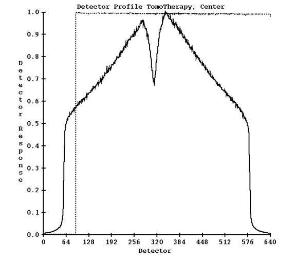
The solid curve is the response of the detectors. The dotted curve is the response of the center detector over all the reads in the detector file. Notice there is an initial warm up time when the detectors are read but x-rays are not on (the leafs are closed). This program does not do anything else.

b) Generate Detector Calibration

Next, from the command prompt window run program GenerateTomoDetector.

You will again be prompted to select the machine and field width. The detector profile above will be compared to the lateral measured profile shown above and a response curve created and written out to file DetectorCalibration25.txt (here for the width 2.5 cm). A plot is shown below:

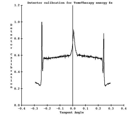
Note for this case, the dip in detector response on where the central axis was is now a peak. The peak in the penumbra region can be ignored or the output file edited. This curve will be applied to all detector readings.

Generating the TomoTherapy Dose Kernel

When all the above data is in for a particular field width, run program FitTomoKernel, again from a command prompt window. The program will fit a spectrum from the % depth dose data, generate the pencil beam kernel (for the particular field width), compute the off axis correction factors from the in water profiles at depth, and compute a calibration constant. The program will also fit the source model and plot the result as shown above. Hit the Enter button again and the program will then compute the dose from the dose kernel and compare to the input data, as shown below:

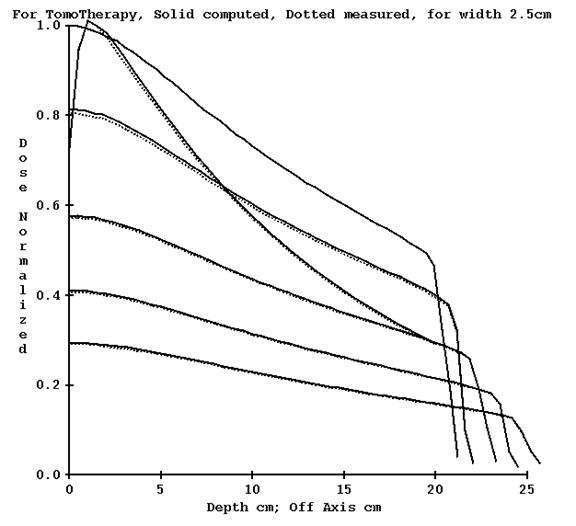
The profiles in water are plotted from the central axis out to one side. Profile data measured has been averaged for each side. The central axis is plotted surface to maximum depth of the data on top of the profile plot.

Absolute Detector Calibration in cGy

The absolute calibration of the detectors is generated from an actual plan. Use a plan that consists of a measurable point in a phantom such as the Cheese phantom to deliver a uniform dose to a region in a cylindrical phantom, where a measurement can be made in the uniform area without any gradients that could affect an ion chamber reading. The water equivalent density of the Cheese phantom should be measured by comparing the transmission through the phantom with the transmission through water for the same energy beam. A biological CT number to density curve might not represent the true water equivalent density of the material in the TomoTherapy beam. A water equivalent value of 1.04 was measured for the Cheese phantom. Set the density of the ROI volume of the phantom to the value measured.

An example plan is shown below with the planning system dose shown (for ten fractions). The dose was measured at dead center.

The detector file is to be measured in a dry run without the phantom and couch in the beam. If the couch cannot be retracted, then a couch correction file must be generated as described below and used.

The tomotherapy couch should be outlined and modeled as described above.

The dose is reconstructed from the pre-treatment detector file and the dose computed by Dosimetry Check at a point is compared to the dose measured at the same point to compute a detector calibration factor.

As an option, a run can also be made with the phantom and couch in the beam to be used later to test the transit dose reconstruction, especially since there is a measured dose.

For an existing plan, you must reselect the detector file to force recalculation with the change in the beam model.

Warning: Keep Final Calibration:

Program SetTomoDetectorCalibration

All detector values are multiplied by a single constant. That constant is to be adjusted so that using the detector values will result in the correct dose being computed in cGy.

Run program SetTomoDetectorCalibration to set the absolute calibration of the detectors. This program will prompt you to select the treatment machine and the field width. For the particular field width, you will be prompted to enter the dose measured at your calibration point for the above calibration plan, and then the dose computed by Dosimetry Check for the same point. The program will then perform the operations describe below for you: adjusting the value in the calibration file and computing the dose conversion constant. The below is for your information.

For example, if measured dose / computed dose = 0.95

then the dose in the calibration file is multiplied by 0.95. Next a new calibration constant in the file TomoDoseConvertConstant25_06 (or corresponding width file) is generated. The calibration constant of 1.254567e-007 in the below example file in affect will then be adjusted (by the same ratio of 0.95 in this example) so that the correct dose will be computed in the future. Alternately one could edit that value directly, but we advise against that as running either FitTomoKernel or ComputeCalConstant will replace the value in that file.

Calibration File

The file TomoCalibration25_06 (name shown for 25 mm field width) is adjusted up or down so that the stated dose in that file will result in the computed test for the above test plan to agree with the measured dose. An example calibration file is shown below. The SSD and depth field are nominal values used for internal purposes and there is no reason to change them.

/* file type TomoTherapy calibration */ 21

/* file format version */ 1

/* machine directory name */ <*TomoTherapy*>

/* energy */ 6

/* date of file: */ <* *>

/* SSD */ 85.0

/* field width cm */ 2.5

/* depth cm */ 1.5

//Dose for calibrated condition in cGy:

447.5

The above dose for the calibration condition would be the dose that is measured in water at the stated point for the exposure as described above for the relative calibration run. The calibration constant is computed so that the detector values will result in the stated dose being computed for the relative detector calibration run. However, because of the narrow field for this condition, it is easier and more accurate to measure the dose in the Cheese phantom than in water with this single exposure, and a test plan is needed in the Cheese phantom anyway to confirm correct commissioning. The measurement in the water phantom is subject to a large uncertainty due to the gradient across the field width (parallel to the axis of rotation) from a single exposure, as compared to making a large homogeneous dose volume in the Cheese phantom for measurement. By adjusting the dose for the calibration condition in the calibration file relative to the result obtained with a test plan, the correct convert constant will be generated with greater accuracy.

TomoDoseConvertConstant

The convert constant is then written to another file TomoDoseConvertConstant25_06 (again the file name shown for the field width of 25 mm), an example file shown below:

/* File type, 102 = dose conversion constant */ 102

// this number converts computed numbers to dose

/* file format version: */ 1

/* machine directory name: */ <*TomoTherapy*>

/* nominal energy MeV */ 6

/* for width cm */ 2.500000

/* dose conversion constant: */ 1.254567e-007

/* date of calibration: */ <*10-Mar-2011-12:13:50(hr:min:sec)*>

Water Transmission Measurements with the TomoTherapy Detectors

The various detectors used in the TomoTherapy machines may have a different energy response as the thickness of water that is in the beam is increased. On different machines we have observed up to a 13% difference in measurement with the detectors as opposed to a calibration therapy ion chamber for 30 cm of water. Below is a plot of detector response versus water thickness from three different machines (red, green, and blue):

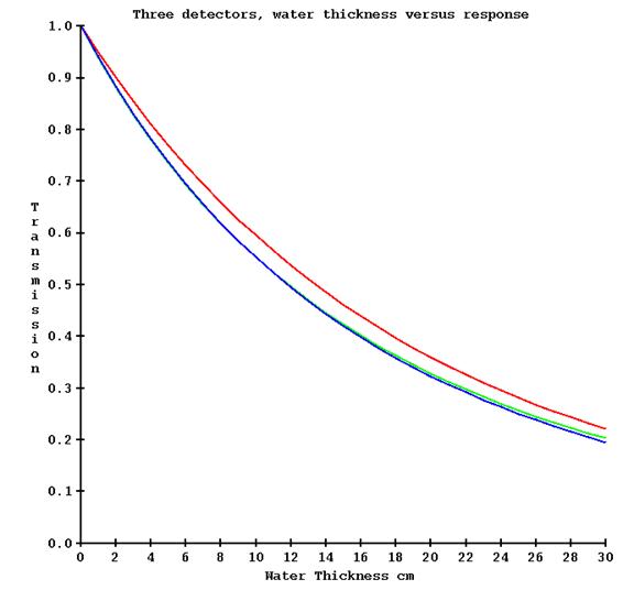
It is necessary to correct for the above detector response if transit dosimetry is to be at all accurate. This is accomplished by making a series of exposures with the no couch in the beam (for a couch attenuation measurement that is not here directly used here), the couch in the beam (for zero water thickness), and then increasing thicknesses of water (include the water equivalency of the tank bottom). The machine must of course be only pointed at the floor. This measurement need only be made for a single field width. By opening the center leafs and then successively leafs further out, the attenuation through water as measured by the detectors can be determined at increasing angles with the central axis.

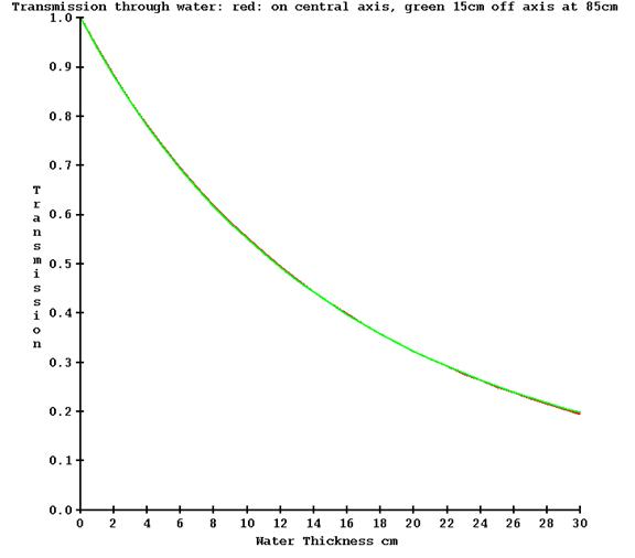
However, there will be little change off axis due to the absence of a flattening filter as compared to a conventional medical linac, but adding off axis measurements does not require any extra work here. Below is a plot of the transmission measured on the central axis (red) and 15 cm off the central axis (green) on a TomoTherapy machine.

For point of comparison, below is the measured transmission on a conventional medical linear accelerator what has a flattening filter, also for 6x, at the same angles off axis:

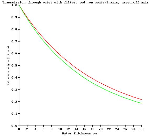
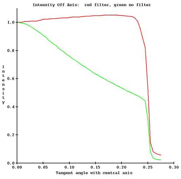
Of course, without a flattening filter the intensity changes a lot more off axis. Shown below is an example of the intensity off axis for the same machine, with and without a flattening filter.

a) Transmission Run File

Our issue here is the first plot above, the response of the detector for the same thickness of water in the beam, which is not to be confused with the other issues. In the below process, it is not any extra effort to measure the transmission off axis, so we include that. To process the data, a run text file must be written that describes the measurements and the detector file obtained for each measurement.

One measurement is to be made without the couch in the beam, then with the couch in the beam. Follow with measurements with increasing amounts of water. The water thickness reported must be the total water equivalent thickness in the beam including the tank bottom but not including the couch since that was measured separately.

An example run file is below:

/* TomoTherapy transmission fit run file */ 23

/* file format version */ 1

/* Machine name */ <*TomoTherapy*>

/* nominal energy */ 6

/* number of channels per row of detector file */ 643

/* number of rows per second */ 10

// leafs open start time end time seconds

// leaf number to

// leaf number.

32 33 30 60

27 28 65 95

37 38 65 95

22 23 100 130

42 43 100 130

17 18 135 165

47 48 135 165

12 13 170 200

52 53 170 200

7 8 205 235

57 58 205 235

9999 // ends the list of leafs and times.

/* time to used as dead time sec */ 2

// no couch in beam file name:

Nocouch.bin

// with couch only file name, this is zero water thickness.

Justcouch.bin

// files with water, total water equivalent cm including

// tank bottom must be in order of increasing water

// thickness.

5cmH2O.bin 5

10cmH2O.bin 10

20cmH2O.bin 20

30cmH2O.bin 30

END

In the file above, leafs 32 to 33 are open from 30 seconds to 60 seconds. Then leafs 27 to 28 are open from 65 to 95 seconds. Also leaves 37 to 38 are open for the same time period. This record describes which leaves are open for what time period of the exposure. By making the openings symmetrical, a measurement can be made on each side of the central axis at the same time. The results for each side will be averaged together below.

b) Program FitTomoTransData

Program FitTomoTransData is run to read this file and fit a water transmission curve. The program does a peak search to find the detectors that are exposed as a refinement to computing which detectors should be exposed, averaging the detector reading between the half intensity points. This data is drawn on a graph, one screen for each thickness Two examples are shown below. The first shows the area measured for leafs at the center (32 and 33):

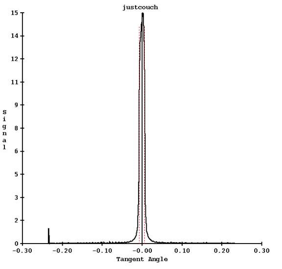
The red dotted line shows the half intensity points between which the detector values are used and averaged.

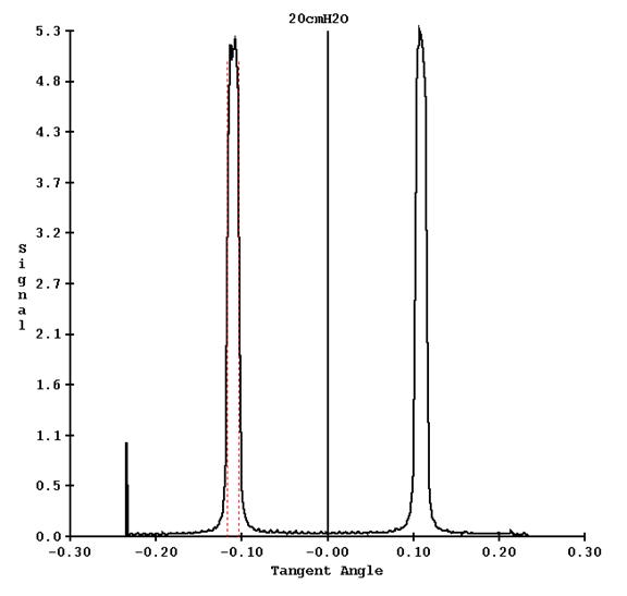
Another example is shown for leafs 17 and 18 from the run file above, for the 20 cm thick water file:

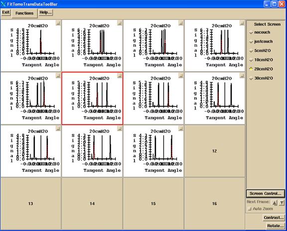
The appearance of the screen is shown for one of the thickness results screen, showing all the frames:

The choices on the Functions pull down are:

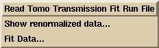
First action is to select to read the run file. The program will popup up a file selection box. The sinogram detector files must be in the same directory as the run file.

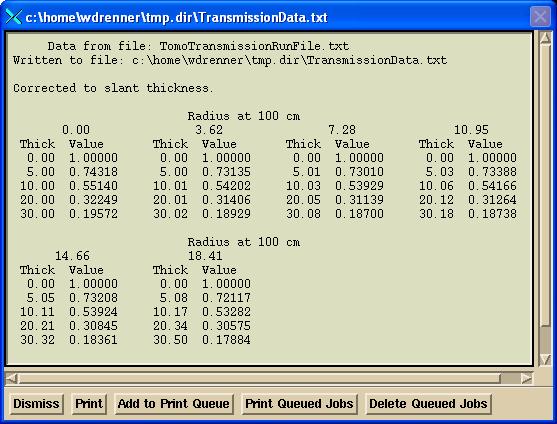
The “Show renormalized data” button will show the transmission data read and computed from the detector sinogram files, normalized to 1.0 for no water (only the couch in the beam). Internally the tangent angles are used. Below the tangents are multiplied by 100 for convenience of reading:

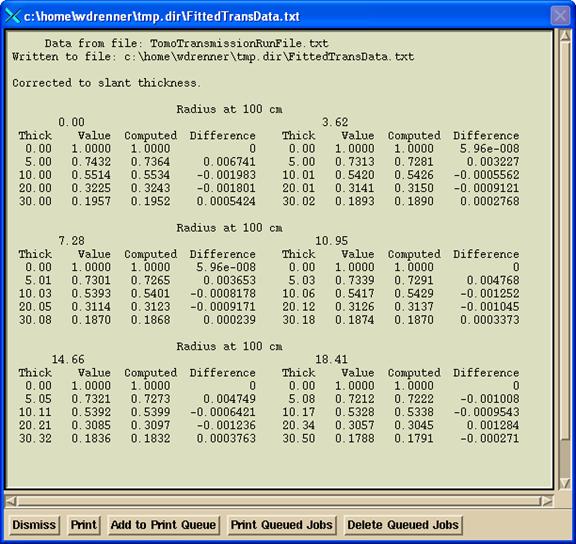
Hit the “Fit Data” will fit four exponentials to each radius. A popup will show the results of the fit:

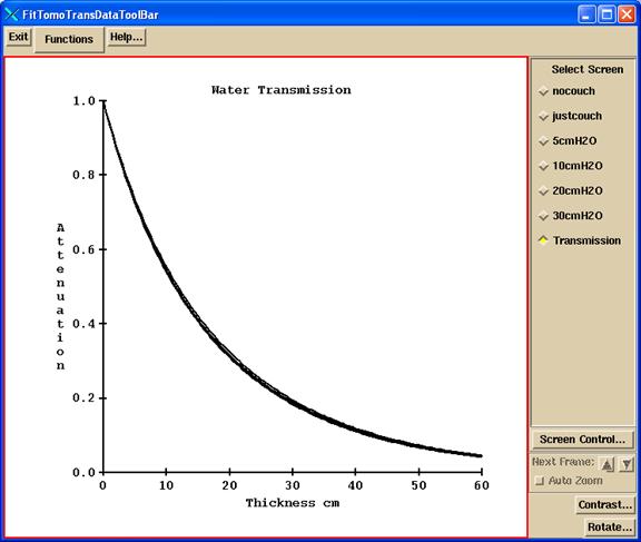
Finally, a graph will be drawn showing the attenuation curves versus thickness for all the radii:

The fitted data is written to the file InWaterTransmissionFit06 in the beam data directory. This file is used to correct for attenuation through the patient to back trace to get the in air fluence. In addition, the file TomoCouchAttenuation.txt is written to show the attenuation measured through the couch by the detectors at each angle. This data is for reference only. Program tools.dir/ComputeThickness.exe can be used to compute the water equivalent thickness from the above InWaterTransmissionFit06 file (run in a command prompt window).

Correcting Pre-treatment Detectors for the Couch In the Beam

If the couch cannot be retracted for pre-treatment images, create or use an xml run file that will rotate the gantry through 480 degrees (360 followed by and additional 120 degrees) to start a 0 degrees and end up at 120, with an integration of the detectors to occur between every angle. Channel cropping must be off. The file size should then be 480 times 4 (the number of bytes in a floating point number) times the number of channels, typically 643, but may be different on different machines, see the Geometry file. Since there are 481 control points, there will be 480 rows of floats in the detector file, one float for each channel.

Run the xml file twice, once with the couch in and once with the couch out of the beam. This is possible in service mode.

Run program TomoPreTreatmentCouchCorrection.exe (from a command prompt window, which will be in the main directory for Dosimetry Check, typically c:\mathresolutions). Select the machine and select the energy (6x is the only choice). Then select the detector file for when the couch was in and then select the detector file for when the couch was out. This is under the Functions pull down on the TomPreCouchCorrection toolbar after selecting the machine and energy as shown below:

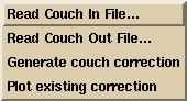
In addition, you must type in the coordinate of the couch height.

Warning: If couch is in, you must use the same couch height for all pre-treatment clinical case runs.

Then select the “Generate couch correction” button. The first 120 degrees of rotation are ignored for warm up considerations. Then for each angle, 0 to 359, the program will compute the ratio between the couch out / couch in for each detector. The program will plot this curve for you to review for each gantry angle. The program will also display the maximum factor observed and the gantry angle it was observed at. You then have the option of enforcing a clamp on the maximum factor. To do so, enter a clamp value and generate the couch correction again for it to take effect.

Shown below is an example correction curve for the detector scan from gantry angle 86 to 87 (hence center of integration is 86.5 degrees).

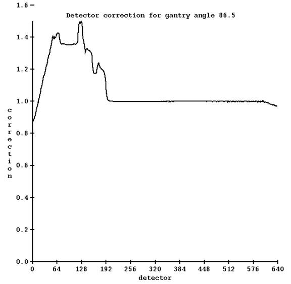
When pre-treatment detector scans are made with the couch in, corrections will be applied for each detector for each angle. If in the clinical run the detector integrates from angle 1 to angle 8, the correction applied will be from the average for the angles 1 to 8, for each detector.

A second screen will show the correction curves for symmetric angles (same rotation from zero but in opposite direction), such as the example below:

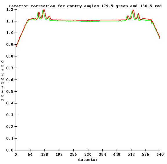
Two files are written by this utility in the energy (X06) folder of the machine:

TomoDetectorCouchCorrection and TomoDetectorCouchCorrectionHeader.txt. The correction will automatically be applied to all pre-treatment detector files.

An example is provided in the below image:

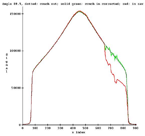
where we are showing a detector scan in black measured with the couch out of the beam, red is the detector scan taken at the same angle with the couch in the beam, and green is the restored curve by applying correction.

a) Couch out of beam for pre-treatment cases.

If at some point the couch can be removed for clinical dry runs, you must delete one or both of the files (or rename them) so that the program will not be able to file the file, and so then not correct detectors for the presence of the couch. The program displays the below popup if it is correcting the detector readings for the couch: