Electron
contamination component
Recommendation
for defining the monitor unit
Collimator in-air scatter factors
Generation
of the Pencil Beam Kernel
Program GenerateBeamParameters
Dose Algorithm
The radiation dose can be computed with a three dimensional dose integration commonly referred to as convolution/superposition or “collapsed cone” (CC), or a two dimensional integration referred to as pencil beam (PB). The CC algorithm is 8 to 14 times slower than the PB algorithm. For this reason computation in dedicated hardware from Nvidia, referred to as a GPU (graphics processing unit), was implemented for both algorithms. The parallel capabilities of the GPU is here put to use strictly for computational purposes. Both algorithms use a variant dose kernel for the purpose of improving the accuracy of the computation. However, that means that the convolution theorem cannot be applied with the Fast Fourier Transform to make the calculation in the frequency domain with the resulting increase in computation speed due to the greater computation efficiency. Hence the calculations are done in the spatial domain, and so the need for parallelism in hardware. For the CC algorithm the kernel is tilted and the path between the interaction points and dose deposition point is scaled by the density along the path. For the PB algoritihm, the depth is scaled by the density for the interaction points.
“Collapsed Cone” Algorithm
The Collapsed Cone Convolution was originally published by Anders Ahnesjo in Medical Physics in 1989 (see list of references below). However, the term collapsed cone has become something of a generic term. What distinguishes his work, in this author’s opinion, is the use of fitting of a derived polyenergetic kernel to equations, and the integration is performed using analytic equations. Electron contamination was not considered. The approximation of energy released into coaxial cones of equal solid angle is essentially the same approximation made in any three dimensional integration that will use evenly spaced angle increments, such as superposition (Mackie et. al. 1985). Our algorithm might be more technically described as convolution/superposition with a variant kernel. The same applies to computing pencil beam in a two dimensional integration and computing the scatter component with scatter air ratios, also in at two dimensional integration.
Convolution kernels computed using Monte Carlo EGS4 code are used to compute monoenergetic depth dose on the central axis (Papanikolaou et. al 1993). Using a functional form (Ali and Rogers 2012) for a photon spectrum, measured depth dose data is used to fit a spectrum beyond the depth of electron contamination. The depth used is found from an iteration for best results, but is less than 10 cm.
A polyenergetic kernel is then computed as a weighted sum of the mono-energetic Monte Carlo kernels. The original data consisted of division into 48 angles. The number of angles is reduced by a factor of 6 to 8 angles by combining the kernel data in the respective cones. Integration is therefore performed in 22.5 degree increments from the direction of the x-ray along the kernel’s Z axis that points to the source of x-rays along diverging rays. In the kernel’s x,y plane, integration is performed every 20 degrees for a total of 18 angles. Hence the total number of cones is 8 x 18 = 144. The kernel is tilted so that the kernel’s Z axis is always pointing toward the source of x-rays. Hence the kernel is variant with position.
Electron contamination component
The polyenergetic kernel is used to compute depth dose for the percent depth dose tables provided for the beam data. Agreement is forced at 10 cm depth by normalization. Shown below is the measured % depth dose in black and the computed photon dose in red for 18 MeV:
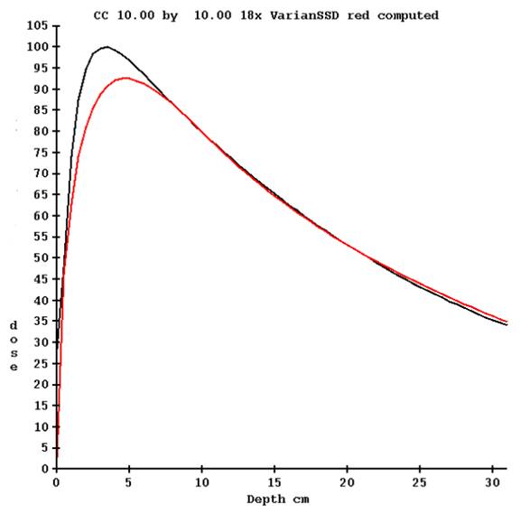
The computed dose is subtracted from the measured dose from zero to 10 cm depth.
From the difference as a function of field size and depth, a pencil beam kernel is derived. This kernel can be thought of as a correction term rather than an electron contamination term, used to compute a correction from 0 to 10 cm depth which accounts for electron contamination. By modeling this as a pencil beam, it can be computed for irregularly shaped and modulated fields. The integration of this term is performed in the plane perpendicular to the central axis at the depth of the point of calculation. For interaction points at and deeper than 10 cm, the contribution is always zero.
Recommendation for defining the monitor unit
Because for the collapsed cone algorithm the dose at dmax is the sum of the computed photon component and the electron contamination component, we recommend that you specify the dose rate in cGy/mu at a depth of 10 cm in the file Calibrationnn (where nn is the nominal energy such as 06 for 6 MV).
If the percent depth dose is 66.8 at 10 cm depth for the calibration field size (typically 10x10 cm) and the dose rate is to be 1.0 cGy/mu at the dmax depth, the dose rate at 10 cm depth would be specified as 0.668 cGy/mu. If defined for some other SSD than 100 cm, then the specification should be so adjusted.
We believe it is good practice to also calibration the machine at 10 cm depth to the specified dose rate. If you think about it, most treatment prescriptions are going to be in the range of 5 to 10 cm depth. Forcing agreement at 10 cm depth will minimize the affect of errors in measured percent depth dose as the depth is changed in either direction.
The below figure illustrates the geometry of the algorithm “collapsed cone” or convolution superposition algorithm.
Figure 1
Photon component
The photon component is computed for each point of calculation by summing the contribution over the 20 angles (theta) in the plane perpendicular to the kernel Z axis (which points toward the source of the x-ray), and then over the 8 angles (phi) from z minus to z plus. Integration proceeds by stepping along the ray from the point of calculation out ward in what is generally referred to as an inverted calculation. The distance along that ray is scaled by the density. The terma is computed to each interaction point from the source. This latter calculation is computed from a pre-computed table of node points along a diverging matrix. At each node the density scaled depth is stored, from which terma is directly computed. For a specific point, the terma is interpolated from the eight corners of the diverging cell that each point is found to be in. This is the same diverging matrix used for the pencil beam algorithm below.
The contribution from all interactions points are added up to give the total dose to the point of calculation. An off axis correction is applied as done for Pencil Beam below. The calculation points are the same nodes at which terma is pre-computed. The dose for an arbitrary point is interpolated from the eight corners of the cell that the point is inside.
Lastly, the dose is corrected by the off axis depth correction as is done with the pencil beam algorithm described below.
Collimator in-air scatter factors
A note on collimator scatter factors computed with “Collapsed Cone” versus Pencil Beam is necessary here. Both the above three dimensional integration (CC) and the below two dimensional integration (PB) use the same Monte Carlo generated mono-energetic kernels. Theoretically for a flat water phantom both algorithms should compute the same thing. However, as indicated above, at dmax a significant portion of the dose is due to electron contamination. But both algorithms take into account electron contamination which enters from the same measured values. How is it that the two algorithms will compute different Sp values, which is the case (see plot below)?
For the pencil beam algorithm, the dose kernel is directly computed from the measured percent depth dose data and the Monte Carlo generated kernels are only used to fill out the pencil beam kernel table to zero radius, 60 cm radius, and 60 cm depth. Electron contamination in implicitly included with the pencil beam kernel as the measured beam data includes the electron contamination. Hence the balk of the kernel is directly derived from measured data, not from the Monte Carlo computed point spread kernels.
For collapsed cone, the photon component is computed directly from the MonteCarlo kernels, with the electron contamination computed with a pencil beam algorithm.
As a result of different computational methods, phantom scatter Sp computed for the same field size differs slightly between the collapsed cone and pencil beam algorithms. The collimator in-air scatter factor Sc is computed from the measured output divided by the computed phantom scatter, and so consequently the Sc factors will differ. This is demonstrated in the below plot which plots in back the Sp factor computed with pencil beam as a function of field size, and the Sp factor computed with the collapsed cone algorithm plotted in red. Bare in mind that at dmax, Sp will also include electron contamination, which is derived from a measured value (albeit the same measured values):
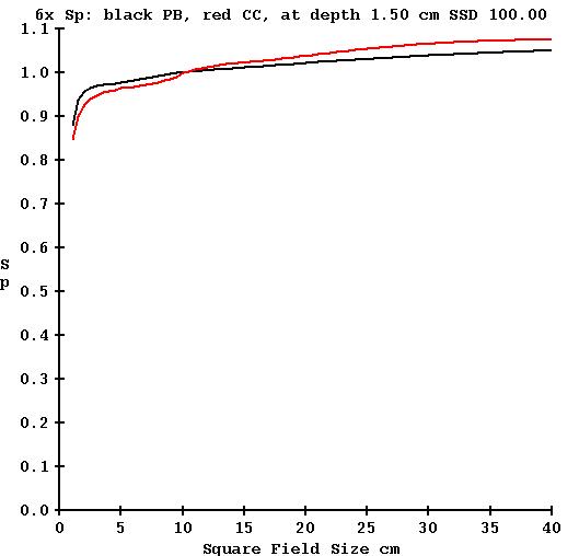
Consequently an EPID kernel derived using Sc values computed from pencil beam would result in small systematic errors if used for a CC calculation and vice versa. If using the pencil beam derived kernel to process images for the CC algorithm, for 5x5 cm field size the dose will be 1.1% too high, and for 20x20 cm field size the dose will be 1.8% too low. Note this refers to open fields. The equivalent field size of modulated fields is generally much less than the size of the border that includes the beam.
Therefore, the EPID kernel must be specific to the dose algorithm to be used to avoid the above small errors.
Algorithm Default File
The file DefaultDoseAlgorithm.txt is the user preference file in the program resources directory (folder) defined by the text file rlresources.dir.loc that is in the current directory. The algorithm is set by the EPID deconvolution kernel and can be over ridden by user selection. The default algorithm file will name the algorithm to use if not set otherwise. In addition, three parameters are specified for the collapsed cone algorithm and are discussed below. Note that only Version 5 release 6 and later of DosimetryCheck will allow setting the start and ending radius increment values.
The number of azimuth angles to integrate in the XY plane of the kernel (the kernel is tilted so that the Z axis points toward the source of x-rays). The value can be set from 8, every 45 degrees, to 36, every 10 degrees. Good accuracy is obtainable with 18 angles, every 20 degrees. The computational time will be directly proportional to the number of angles. Using 8 azimuth angles will give the fastest compute time, but there can be variations up to 2% among points computed. Consider the rays every 45 degrees emitting from a point and where they will intersect the boundaries of the edges of a field. Integration is along those rays. The number of zimuth angles is fixed to 8, every 22.5 degrees. The number of cones is 8 times the number of azimuth angles.
The pencil beam has 36 azimuth angles for IMRT, 18 for IMAT and is hard coded.
For the collapsed cone algorithm, control is provided for the integration increment along the radius. The starting increment a 0 radius and increment at 60 cm is specified. The increment is ramped between 0 and 60 cm. The increment is first ramped at the radius of 2.5 cm and then every 5 cm there after. For the default 0.5 cm matrix spacing (see the file DefaultCalculationMatrixSpacing.txt below), the radius increment can start at 0.5 cm and end at 2.0 cm for reasonable accuracy. For a finer matrix spacing of 0.2 cm, a finer radius increment to obtain smooth looking dose curves is needed. 0.1 cm to 1.0 cm will serve that purpose. However, the computer time will increase by a factor of 3.4 over 0.5 to 2.0 cm.
An example file DefaultDoseAlgorithm.txt is shown below (and can be copied to make the text file). See also the ASCII file format specification rules in the System2100 manual.
/*
file format version defines what is below */
3
// Below specify the default dose algorithm to
use:
// 0 for Pencil Beam, 1 for collapsed cone 1
//
for collapsed cone: number of azimuth
angles: 8 to 36
//
default is 18, recommend 18
18
//
for collapsed cone: start increment for integration along
//
radius in cm, 0.1 to 0.5 cm. Default
is 0.1 cm
0.5
// final size of step at radius of 60 cm, max is
2.0 cm, default 1.0
2.0
//
calculation time increases with the number of azimuth angles
//
and increases with decrease in start increment.
//
For 0.5 cm dose matrix size recommend 18 azimuth angles and
//
0.5 to 2.0 step size in radius.
//
for 0.2 cm dose matrix size recommend 18 azimuth angles and
//
0.1 to 1.0 step size.
The file DefaultCalculationMatrixSpacing.txt is also shown below:
/*
file format version */ 1
//
file to specify the default matrix spacing for calculation of dose
//
spacing in the plane perpendicular to the central axis in cm
//
minimum 0.1 cm, maximum 2 cm
0.50
// spacing
along the diverging rays in cm
//
minimum 0.2 cm, maximum 2 cm
0.50
//
for rotating beams with fixed field shape or fluence file
//
increment to simulate a rotating beam in degrees (integer only)
//
minimum 1, maximum 20
10
Note that the above rotation increment is for the case of rotating a non-changing radiation field. For IMAT (VMAT, RapidArc), the rotation is simulated by the EPID images, one beam for each EPID image at the angle the EPID image is integrated at.
Pencil Beam Algorithm
|
Figure 2 |
Below we will give details on how the pencil beam is developed from measured beam data and Monte Carlo calculated kernels. A single poly-energetic kernel is used to represent the pencil. There were two considerations for making this choice. First we would like the algorithm to be as fast as possible. Calculating each energy separately with a spectrum and mono-energetic kernels would reduce the speed significantly. Second, for the Dosimetry Check application, we have to consider the input information. We can only measure dose in a plane perpendicular to a beam, not the spectrum, at individual pixels covering the radiation field. Therefore we need an algorithm that can start with the intensity distribution in reference to dose.
|
Figure 3 |
The dose is computed to the point P according to the below formula. r is the radius at depth from point P to the differential area element dr rdq. (x,y) is the coordinates of P at the treatment machine’s isocentric distance Sad. (xr,yr) is coordinates of the differential area element at distance Sad.


where
In words, dose_c is the computed constant that converts everything that follows to give the calibrated dose for the calibration field size, SSD, and depth. The units of the pencil kernel therefore do not really matter. Dose_c is simply the ratio of the specified dose rate, usually 1.0 cGy/mu, for some field size, SSD, and depth, to the result computed for the same field size, SSD, and depth.
The Off Axis Correction table is developed from measured diagonal fan line data taken at depth for the largest field size. This two dimensional table is simply the ratio of measured over computed values stored as a function of the tangent of the angle with the central ray, t above, and depth. The depth de is the effective depth of the point of calculation P. de is computed by tracing along a ray from the point of entry into the patient body, and summing the incremental path length times the density at the location. This table provides a means of accounting for the change in beam penetration off axis since the kernel was developed from data on the central ray.
The Sad/Spd squared term is the inverse square law, where Sad is the source axis distance of the treatment machine, typically 100cm. Spd is the distance from the source to the plane point P is in, along the central ray.
Next follows the integration of the pencil beam kernel over the area of the field. This formula is of course only symbolic. We can only integrate numerically on a computer, but the formula does show the mathematical idea. The kernel K(r,de(r,q))/2pr is the dose at the radius r at depth to the point P from the incremental area dr rdq. de(r,q) in cylindrical coordinates centered at P equals de(xr,yr) in Cartesian coordinates and is the equivalent depth along the diverging ray through the differential area element at the surface to the plane perpendicular to the central ray that contains the point P. We actually don’t have this kernel K, what we do have is the integration of K from 0 to r which is the dose at P from the circular disk of radius r at depth. So we actually take a difference here over dr in the numerical computation. Note that the r term cancels out and we have taken the 2p term outside of the integral.
The differential area element is weighted by the field intensity Field at (r,q), here shown in the Cartesian coordinates (xr,yr) at the distance Sad. For the Dosimetry Check program, this is looked up directly from the pixel value at that location from the measured field. In comparison, program GenerateFieldDoseImage computes this value at each pixel location as the product of the monitor units, the scatter collimator factor, the in air off center ratio table, and the attenuation of any shielding blocks. For general treatment planning we would here also model the attenuation of any wedge, compensators, and any other devices that effect the field fluence such as a multi-leaf collimator.
The one over the maximum of one or the in air off axis ratio (OCR) term is to correct the kernel for having been derived from data that contains the effect of the OCR. Here we divide it out as long as the OCR has a value greater than one. The effect of most flattening filters on the OCR is that the in air fluence increases initially with radius. We want to correct for that effect. Otherwise for points on the central axis we could be effectively applying the effect of the OCR twice during integration over the area of the field, once built into the kernel and then formally through the above Field term.
But in the corner of the largest field the OCR value often decreases due to a cut off of the field due to the primary collimator. We do not want to cancel out that effect in those areas. The correction here is a compromise to achieve some deconvolution of the OCR term out of the kernel term. As the OCR is stored in terms of the tangent angle a ray makes with the central ray, we divide the radius at depth by the SSD used to measure the fields from which the kernel was derived plus the effective depth along the ray from the differential area element to the plane perpendicular to the central ray that contains the point of calculation P.
Note that there are two effective depths used in the above equation. One is along the ray to the point of calculation P, de(x,y). The other is inside the integration (sum) and is traced along the ray from the surface to the differential area element dr rdq = de(xr,yr). The ray tracing along each ray is only done once. A fan line grid covering the area of the beam is created. Each fan line is ray traced through the patient with the storing of the accumulated equivalent depth at intervals along each ray. The spacing between the fan lines is set at a level half way through the patient to the dose matrix spacing value that the user can reset from the default value. Below this plane the fan lines are diverging further apart and above the plane the fan lines are converging closer together. Node points are distributed along the fan lines at equally spaced intersecting planes perpendicular to the central ray, and it is at these node points that the equivalent depths are stored. During the above numerical integration over each plane, the nearest ray is used to look up the equivalent depth. The same node points that hold the equivalent depths also define the points to be calculated. All other points are interpolated within this diverging matrix.
Let us note here the approximations that are made. The integration is in the plane perpendicular to the central ray that contains point P. Rigorously it can be argued that the integration should be in the plane perpendicular to the ray from the source to the point P. For a worst case, the largest field size of 40x40, the ray at the edge of the field on a major axis makes an angle of 78.7 degrees instead of 90 degrees, an 11.3 degree difference, which is not going to make a large difference. The Off Axis Correction above will tend to cancel out such approximations. To be consistent, the Off Axis Correction is computed using the same algorithm. Using the inverse law correction for the slant depth along the ray from the source to point P made no difference from using the vertical distance parallel to the central ray. Another approximation is made below in the generation of the pencil kernel. It is assumed that at a depth d and radius r, the dose will be the same for a cylinder of radius r and for a diverging cone of radius r at the same depth. This is the same approximation made in the concept of Tissue Air Ratio.
Rectangular arrays of equally spaced points are generated for planar images, and a three dimensional lattice of points is generated for 3d perspective room views. The dose at these points are computed for each beam by interpolating within the above diverging fan line array of points generated for each beam. This means that in general the dose is interpolated between the eight corners of the diverging box that a point is inside. We will interpolate with less than eight points provided that the sum of the weights from the points is greater than 0.5, as some node points might fall outside of the patient. Once computed, each beam saves its dose matrix to a disk file, unless the beam is changed in which case a new fan line dose matrix array is created.
Generation of the Pencil Beam Kernel
Program GenerateBeamParameters computes the pencil kernel from measured data (and has been updated to also generate the polyenergetic point kernel for the collapsed cone algorithm). It does this in a two step process. We started with Monte Carlo computed mono-energetic point spread functions. We used those to compute mono-energetic pencil beam kernels. Next we take the central axis data at different field sizes to fit a spectrum.
Note: version 6 release 3, 22 Feb 2018 of GenerateBeamParameters and there after uses the form for the spectrum as is used for the collapse cone above. Prior to this, the below Guassian form is use.
We constrain the spectrum to be a smooth curve by using a Guassian (or normal) distribution, with the spread parameter different before and after the peak value, giving for parameters to be fitted: the peak energy value E0, the magnitude of the peak value A, the spread before the peak sl and the spread after the peak su. The collapsed cone algorithm uses a functional form (Ali and Rogers 2012) for the photon spectrum.
where
Using these kernels and spectrum to compute the dose, the
dose at the surface is necessarily zero, whereas contamination electrons will
result in some dose at the surface. At
lower energy such as 6 MeV, the fitted spectrum with
For these reasons we instead generate a poly-energetic pencil kernel. The above fitted spectrum and mono-energetic pencil kernels are used for three purposes:
One, at 10 cm depth, which is beyond the range of contamination electrons, we can compute phantom scatter. This provides a means of separating the scatter collimator factor from the measured output factor for each measured field.
Two, we can compute the equivalency of circular fields to square fields, again at 10 cm depth, and use the resultant table to assign equivalent radii at each depth to the table of measured percent depth dose and square field sizes. We may now calculate an accumulated pencil kernel as a function of radius and depth from the measured square field percent depth dose data.
Three, we can complete the poly-energetic pencil kernel to zero field size, to a depth of 60 cm, and to a radius of 60 cm (the range for which the mono-energetic kernels cover), by scaling the results of the mono-energetic kernel and spectrum to agree where the tables join. From the surface to dmax the curvature computed at dmax is simply scaled to fit the end points from the smallest field and largest field in extending to zero radius and 60 cm radius respectively.
In this manner we produce a poly-energetic kernel which by design returns the same percent depth dose for all depths and field sizes measured.
Program GenerateBeamParameters
This program generates both the pencil beam kernel and the point spread kernel for the collapsed cone algorithm.
This program performs the above function of first fitting the spectrum and then using the result to assist in forming a poly-energetic kernel from measured beam data. After the poly-energetic kernel is created, this program computes the Off Axis Correction table from data measured in water along the diagonal of the largest field size at different depths. Next the program computes the dose using the specifications for field size, depth, and SSD for the calibration definition and uses the result to compute the normalization constant that will convert computed results to cGray/mu. Lastly, the collimator scatter factor is computed by dividing computed phantom scatter into the output measured for each field size. The collimator scatter factor is used by program GenerateFieldDoseImage to compute the equivalent of a measured field which is to be used for testing purposes.
This program is an ASCII run program, meaning you run it in an xterm window with keyboard commands. The program will prompt you to select the treatment machine and then the energy. The program will take several minutes, most of the time spent in the initial step of fitting a spectrum. The program will stop if an error occurs, such as a needed file is missing. Be sure to check for error messages when the program has finished to ascertain that it was successful in computing all the output files that are required.
Program ComputePolyCAFiles
This is an ASCII program that will compare the dose in the central axis data files to that computed using the pencil beam or the collapsed cone dose algorithm. A report is produced that can be printed on a printer. A plot for each field size comparing the measure data to computed data is produced. This is an ASCII program that must be run from the keyboard in a command prompt (xterm) window. It provides a test that the kernel was properly generated. The program works for both the pencil beam algorithm and the collapsed cone.
References
1. T.R. Mackie, J.W. Scrimger, J.J. Battista, “A Convolution Method of Calculating Dose for 15-MV X-Rays”, Med. Phys., Vol. 12, No. 2, Mar/Apr 1985, pp 188-196.
2. A. Ahnesjo, “Collapsed cone convolution of radiant energy for photon dose calculation in heterogeneous media”, Med. Phys. Vol. 16., No. 4, Jul/Aug 1989, pages 577-592.
3. M.D. Altschuler, P. Bloch, E.L. Buhle, S. Ayyalasomayajula, “3D Dose Calcuations for Electron and Photon Beams”, Phys. Med. Biol., Vol. 37, No. 2, 1992, pp 391-411.
4. N. Papanlkolaou, T.R. Mackie, C. Wells, M. Gehring, P. Reckwerdt: “Investigation of Convolution Method for Polyenergetic Spectra”, Med. Phys., Vol. 20, No. 5, Sept/Oct 1993, pages 1327-1336.
5. P.A. Jursinic, T.R. Mackie, “Characteristics of Secondary Electrons Produced by 6, 10, and 24 MV X-Ray Beams”, Phys., Med. Biol., Vol. 41, 1996, pp 1499-1509.
6. P. Bloch, M.D. Altschuler, B.E. Bjarngard, A. Kassaee, J.M. McDonough, “Determining Clinical Photon Beam Spectra from Measured Depth Dose with the Cimmino Algorithm”, Phys. Med. Biol, Vol. 45, 2000, pp 171-183.
7. A.L. Medina, A. Teijeiro, J. Garcia, J. Esperon, “Characterization of electron contamination in megavoltage photon beams”, Med. Phys. Vol. 32, No. 5, May 2005, pages 1281-1292.
8. E.S.M. Ali, D.W.O. Rogers, “Functional forms for photon spectra of clinical linacs”, Phys. Med. Biol, Vol. 57, 2012, pages 31-50.
9. E.S.M. Ali, D.W.O. Rogers, “An improved physics-based approach for unfolding megavoltage bremsstrahlung spectra using transmission analysis”, Med. Phys. Vol 39, No. 3, March 2012, pages 1663-1675.
Acknowledgments
The author would like to here acknowledge the assistance
provided by Dr. Thomas (Rock) Mackie of the