It may be suitable for the Dosimetry Check program to use generic beam data. The generic data provided can be copied to create a machine. It might then be only necessary to edit the geometry file specifying the geometric parameters of the treatment machine and for each energy, the calibration file. The supplied generic data provides templates for modifying or creating beam data for a particular machine. A useful utility program is ReplaceText that will replace found text with a different string, to change the machine name in files if building a beam data file system from a template. After editing the calibration file, be sure to run program ComputeCalConstant.

All the files are ASCII text files and are self documenting. Numerical information is off set with white space. Text fields that programs are to read are set off between the symbols <* and *>. If there are no spaces (white space) in the text string the text need not be delineated with the above symbols. A comment line is set off with two slashes to the end of the line. Or a comment may be enclosed between /* and */ which can be nested. When reading a file programs ignore the comments.

Utilities may exist to copy existing beam data in other formats to the file structure required here. Program ConvertRenBeamFiles, for example, will copy the ASCII beam data files used for Render-Plan 3-D from Elekta Oncology to our file format. This is an ASCII program run in an xterm. Just invoke the name of the program, the directory where Render-Plan beam data files are, and the directory where the data files are to be copied and transformed to. We expect to write these utilities on a need bases as people supply us with examples of their beam data.

All beam data resides in the directory specified by the file BeamData.loc in the program resources directory. Each treatment machine is represented by a subdirectory. In the subdirectory are files containing information common to the treatment machine. Each energy will have a subdirectory, for example X06 for 6 MV x-rays, X18 for 18 MV x-rays. We will here give examples of these files.

The Generate Beam Parameters Program

Program GenerateBeamParameters will read the below input files and write output files. The output files are not documented here. Those files that are ASCII are self documenting however. There should normally be no reason to edit the output files, but they might supply useful information. The kernel files are stored as binary files. This program is described above in the Algorithms section.

Machine Description File

This file simply holds a text description of the treatment machine.

Example file name: Description

Example file:

/* file format version: */ 1

<* SL20, 6 and 18 MeV x-rays*>

Machine Geometry File

This file defines the geometry of a treatment machine.

Example file name: Geometry

Example file:

/* file format version: */ 2

/* Source Axis Distance (cm) = */ 100.00

// This is also the distance field sizes are defined at.

/* largest field size (cm) is */ 16 21

In formation version 2 above, two numbers are expected for the maximum field size, which would be 40 40 in normal cases, but there is a machine where it is 16 by 21. The first number is the size long beam’s eye view X axis, and the second along the Y axis.

Below is the prior format, the rest being the same:

/* file format version: */ 1

/* Source Axis Distance (cm) = */ 100.00

// This is also the distance field sizes are defined at.

/* largest field size (cm) is */ 40.00

/* Positive gantry rotation: +1 = clockwise, -1 = counter-clockwise */ -1

/* Gantry angle value when pointed at floor: */ 180.00

/* Positive collimator rotation: -1 = clockwise viewed from ceiling

+1 = counter-clockwise, with accelerator pointed at floor */ -1

/* collimator nominal angle value = */ 180.00

/* collimator rotation lower limit = */ 83.00

/* collimator rotation upper limit = */ 275.00

/* Positive couch rotation: -1 = clockwise viewed from ceiling

+1 = counter-clockwise */ 1

/* couch nominal angle: */ 180.00

/* X axis, positive couch lateral direction, positive is +x IEC (when moves to your right looking toward the gantry)

Enter opposite sign here */ -1

/* center position value (cm) */ 0.00

/* Y axis, positive couch longitudinal direction, positive is +y IEC (when moves toward gantry)Enter opposite sign here */ -1

/* center position value (cm) */ 0.00

/* Z axis, positive couch height direction, positive is +z IEC (when moves up) Enter opposite sign here */ -1

/* center position value (cm) */ 0.00

/* 1 = lower jaws are X jaws (move sideways),

2 = lower are Y jaws (move front to back) */ 1

/* Independent jaws: 0 = neither, 1 = X jaws (left to right)

2 = Y jaws (front to back), 3 = both */ 2

/* label for -X jaw: */ <*X1 *>

/* label for +X jaw: */ <*X2 *>

/* label for -Y jaw: */ <*Y2 *>

/* label for +Y jaw: */ <*Y1 *>

/* limit of travel for each independent jaw, given as a coordinate in cm

-x jaw +x jaw -y jaw +y jaw */

0.00 0.00 10.0 -10.0

List of X-ray Energies

This file holds the list of x-ray (photon) energies available on the treatment machine. Each energy will have a subdirectory, for example X06.

Example file name: Photons

Example File

/* file format version: */ 1

/* number of photon energies: */ 2

6 18

Central Axis Beam Data

This file is to hold data on the central axis for square fields and resides in the energy subdirectory. Generally the SSD should be the same as the isocentric machine, typically 100 cm. All the central axis files should have measurements at the same depths.

Example file name: CA12.0x12.0_w00_06

Example file:

/* file type: 2 = Central Axis */ 2

/* file format version: */ 1

/* machine directory name: */ SL20

/* energy = */ 6

/* date of data: */ <*25-AUG-1996 11:22:24*>

/* wedge number, 0 = no wedge */ 0

/* field size in cm = */ 12.00 12.00

/* Source to Surface Distance in cm = */ 100.00

/* Number of depths: */ 47

/* depth cm value*/

0.00 46.680000

0.50 73.089996

1.00 95.760002

1.50 100.120003

1.60 100.000000

2.00 99.199997

3.00 95.699997

4.00 92.080002

5.00 87.470001

6.00 83.660004

7.00 79.959999

8.00 76.150002

9.00 72.550003

10.00 68.930000

...

39.00 15.430000

40.00 13.880000

42.50 12.170000

45.00 10.740000

47.50 9.440000

Note that the file starts with a file type field that defines this file as a central axis data file. The file format version that follows defines the format version of this type of file. If the type of data that this file holds must change in the future, we can simply define a different format. The machine name and energy follows. One will not be able to move files around between machines without changing the machine name here. This is the directory name under which the files are stored. The values are generally normalized to 100.0 at dmax.

Central Axis File List

This file contains the list of central axis files.

Example file name: CAFileListw00_06

Example file:

/* file type: 7 = list of CA files: */ 7

/* file format version: */ 1

/* machine directory name: */ SL20

/* nominal energy = */ 6

/* wedge number = */ 0

CA03.0x03.0_w00_06

CA04.0x04.0_w00_06

CA05.0x05.0_w00_06

CA06.0x06.0_w00_06

CA08.0x08.0_w00_06

CA10.0x10.0_w00_06

CA12.0x12.0_w00_06

CA15.0x15.0_w00_06

CA20.0x20.0_w00_06

CA25.0x25.0_w00_06

CA30.0x30.0_w00_06

CA35.0x35.0_w00_06

CA40.0x40.0_w00_06

// Depths measured should be all the same.

This file is consulted when the data from separate central axis files need to be pooled together to create a table of field size versus depth dose, such as when creating the pencil beam kernel.

Dmax File

This file simply defines the depth of dmax for the particular energy.

Example file name: Dmax06

Example file:

/* file type: 3 = dmax value */ 3

/* file format version: */ 1

/* dmax in cm = */ 1.60

Field Size Output File

This file holds the measured output for field sizes.

Example file name: OutPut06 or Output_w00_06 (were w00 is for zero wedge, meaning no wedge)

Example file:

/* file type: 5 = output factors */ 5

/* file format version: */ 1

/* machine directory name */ SL20

/* energy */ 6

/* date of file: */ <*25-AUG-1996 11:22:24*>

//Normally only square fields.

// cm cm cm cGy/mu

// field size SSD Depth output factor

3.00 3.00 100.00 1.60 0.891000

4.00 4.00 100.00 1.60 0.910000

5.00 5.00 100.00 1.60 0.921000

6.00 6.00 100.00 1.60 0.933000

8.00 8.00 100.00 1.60 0.953000

10.00 10.00 100.00 1.60 0.969000

12.00 12.00 100.00 1.60 0.985000

15.00 15.00 100.00 1.60 0.998000

20.00 20.00 100.00 1.60 1.021000

25.00 25.00 100.00 1.60 1.034000

30.00 30.00 100.00 1.60 1.044000

35.00 35.00 100.00 1.60 1.049000

40.00 40.00 100.00 1.60 1.051000

The dose rate for the calibration field size must be consistent with the calibration file to follow and note the values are in cGy/mu and are NOT simply normalized to the calibration field size.

Calibration File

This file holds the definition of the machine calibration.

Example file name: Calibration06

Example file:

/* file type: 4 = calibration */ 4

/* file format version: */ 1

/* machine directory name */ SL20

/* energy */ 6

/* date of calibration: */ <* 31-JUL-1996 13:39:24 *>

/* calibration Source Surface Distance cm: */ 98.40

/* calibration field size cm: */ 10.00

/* calibration depth cm: */ 1.60

/* calibration dose rate (cG/mu) : */ 1.000

Note that this machine is calibrated isocentrically 100 cm to the detector, hence 98.4 cm to the surface. The specification also could have been to a source surface distance of 100.0 with a dose rate of 0.969 cG/mu.

Calibration constant

If your machine’s calibration is different from the generic beam data provided, you need only edit the above file and then run program ComputeCalConstant for the new calibration specification to be used. Alternately you can run program DefineMonitorUnit to both edit the calibration file and compute the conversion constant. The constant is written to the file DoseConvertConstant.

Diagonal Fan Line File

This file holds data measured on the diagonal of the largest field size. Rather than store the off axis distance, the tangent of the angle the ray makes to the central axis is stored. Typically this is just the off axis distance divided by 100. Note however, that this does not have to be measured at 100 cm SSD, but could be measured at a shorter distance. Otherwise a data acquisition system could have the central axis off set to one corner of the tank so that scans can be made along one diagonal. The field size refers to the jaw opening and is the field size at the isocentric distance of the machine, typically 100 cm. If possible data for more than one diagonal should be averaged. This data is used to compute the off axis correction factor which accounts for the change in beam penetration off axis due to the change in energy spectrum off axis.

The depths in the table may be specified and measured as the vertical depth or slant depth. If vertical than all the data at each depth lie on the same plane. If slant than the data for the same depth lie on an arc. Most data acquistion systems would measure the off axis scans on the same plane.

The off axis data stored here starts with the central ray and goes on a 45 degree diagonal to the corner of the field. An increment of 1 or 2 cm is good. All the data for each off axis point must fall on diverging fan lines.

Example file name: DiagFanLine40.0_w00_06

Example file:

/* file type: 6 = Diagonal Fan Line */ 6

/* file format version: */ 1

/* machine directory name: */ SL20

/* energy = */ 6

/* date of data: */ <*25-AUG-1996 11:22:24*>

/* wedge number, 0 = no wedge */ 0

/* field size in cm, x direction, y direction = */

40.00 40.00

/* Source to Surface Distance in cm = */ 100.00

/* 1 = slant depth, 2 = vertical depth */ 1

/* Number of depths: */ 41

/* Number of radii: */ 15

// depth cm tan = radius/distance

0.0000 0.0200 0.0400 0.0600 0.0800

1.65 1.00000 1.01010 1.01710 1.02360 1.03420

2.00 0.99030 1.00390 1.01130 1.01610 1.02680

2.50 0.97490 0.98820 0.99640 1.00060 1.01110

...

34.00 0.23360 0.23810 0.23990 0.23950 0.23860

35.00 0.22290 0.22710 0.22870 0.22820 0.22740

// depth cm tan = radius/distance

0.1000 0.1200 0.1400 0.1600 0.1800

1.65 1.05310 1.05680 1.06180 1.06400 1.06200

2.00 1.04580 1.04910 1.05280 1.05620 1.05400

2.50 1.02760 1.03030 1.03330 1.03720 1.03700

...

34.00 0.23360 0.23810 0.23990 0.23950 0.23860

35.00 0.22290 0.22710 0.22870 0.22820 0.22740

// depth cm tan = radius/distance

0.1000 0.1200 0.1400 0.1600 0.1800

1.65 1.05310 1.05680 1.06180 1.06400 1.06200

2.00 1.04580 1.04910 1.05280 1.05620 1.05400

2.50 1.02760 1.03030 1.03330 1.03720 1.03700

...

33.00 0.21530 0.19790 0.16270 0.05830 0.03100

34.00 0.20370 0.18790 0.15470 0.05550 0.02970

35.00 0.19400 0.17770 0.14680 0.05320 0.02860

In Air Off Center Ratio File

This file holds the off center ratio measured in air. Typically one will put a build up cap on an ion chamber, and measure the dose on the diagonal of the largest field size. The diagonals should be averaged with the data starting on the central axis and going to the corner of the field. The off axis distance is in terms of the tangent the ray makes with the central ray.

Example file name: InAirOCR06

Example file:

/* file type: 8 = In Air OCR */ 8

/* file format version: */ 1

/* machine directory name: */ SL20

/* energy = */ 6

/* date of data: */ <*25-AUG-1996 11:22:24*>

/* Number of data pairs: */ 33

// Must be in increasing order, starting with central axis

// Tangent OCR

0.00000 1.00000

0.00980 1.00750

0.01960 1.01730

0.02930 1.02390

0.03910 1.02580

...

0.26400 0.07470

0.27370 0.04780

0.28350 0.03930

0.29330 0.03270

0.30310 0.02770

0.31280 0.02270

Conversion Utilities

Programs have been written to convert data written by beam data acquisition systems to the format needed by Dosimetry Check (and RtDosePlan for the same files involved), but are not documented here. However, it seems that the format changes with the version of the software of the particular system and there is not a common standard. However, recently those systems are able to write to Microsoft Excel, and this will provide us a common format to input. We will describe three programs that can be used to read data into our beam data format:

ConvertMSExcelPDD: for reading in in water percent depth dose data.

ConvertMSExcelDiag: for reading in in water diagonal scan data.

ConvertInAir: for reading in in air diagonal scan data.

However, none of these program directly reads a Microsoft Excel file. Rather you have to save a sheet in text format and read the text file. All three programs are ASCII programs that must be run in a command prompt window. Run the programs from the main directory where DosimetryCheck is installed, typically in Windows this is c:\mathresolutions. C:\mathresolutions contains dll files needed by Microsoft programs. An alternative is to add the path c:\mathresolutions to the system paths so that c:\mathresolutions will be searched for dll files during run time. On linux, this is not an issue. The program are stored in the directory tools.dir. To invoke the programs type:

tools.dir\ ConvertMSExcelPDD.exe path_to_file_to_read

where the second argument is the path to the input file to be read. If you do not enter a second argument, then the program will prompt you to enter a path to a file later on in the program. In linux, it is tools.dir/ConvertMSExcelPDD, etc..

Upon running the programs, the programs will prompt you to choose the accelerator from the list in the beam data directory, and the list of energies. Therefore you must have first created a directory entry and in that directory and then created a Geometry file and a Photons file. For each energy listed in Photons you must create a directory: X06 for 6x, X18 for 18x, for example.

Windows Mouse in Command Prompt Windows

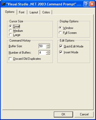
In Windows you can avoid typing by right clicking on the title bar of the command prompt window and select Properties:

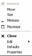
Then on the Properties popup select Quick Edit Mode

This will allow you to high light text with the left mouse. Clicking with the right mouse once will copy it, and clicking with the right mouse afterwards will deposit this text in any command prompt window. Control V will deposit in a Windows window, such as Word or Excel. Also don’t forget the up arrow key will retrieve prior commands you have typed in.

Linux Mouse in X terminal Command Prompt Windows

In linux and unix, you only need to high light text with the left mouse. Middle mouse will then deposit the text elsewhere. Also don’t forget the up arrow key will retrieve prior commands you have typed in.

Converting percent depth dose files

Program ConvertMSExcelPDD.exe will prompt you to enter the SSD and nominal depth for dmax for the data below.

The file must be edited to have the below format. Either do this in Excel and the save as a text file or edit the text file. The first line read is as below with the word “Depth” in it:

Depth (cm) 2 X 2 cm 3 x 3 cm 4 X 4 cm 5 X 5 cm 6 X 6 cm 7 X 7 cm

There may not be lines of data above the line with the word “Depth”. The program reads lines until it finds a line with the word “Depth” and assumes that line is the beginning of the percent depth dose table. After the word “Depth” may be cm or mm which will designate whether the column under depth is the depth in cm or mm.

The field sizes are listed in the rest of the line. There must be a ‘x’ or ‘X’ between each dimension of the field size. The field size must be in centimeters. All other text in the line is ignored, so the following cm in the above example is ignored. The program looks for numbers only and is expecting two numbers for each column of data. This line can wrap on your text editor but is assumed to end with a new line. The entire table can be in one unit, with lines too long for your text editor too show as one line as long as the lines are wrapping around and there is not a new line within a line of data.

The percent depth dose data follows on the next line (no blank lines in between). The data does not have to be arranged in neat columns. All that matters is that each line of data contain the depth in the first field, and a percent depth dose for each field size in the above line. It does not matter how the data is normalized as it will be renormalized to 100 at dmax when printed out. In the below we see depths of 0.0 cm, 0.1 cm, and 0.2 cm. Since there are six field sizes above, there must be data for six field sizes.

0.0 47.87 50.98 49.71 52.58 54.41 55.71

0.1 53.77 56.99 55.78 59.25 61.28 61.97

0.2 60.53 63.6 64.21 67.75 69.65 70.08

The last depth should either be followed by the end of the file or a blank line.

After the blank line you can continue the table with more field sizes if the data is not in a single table unit, for example:

8x8 10x10 15x15 20 x 20 30X30 40x40

The data must follow as above, starting with the depth value. The list of depths must agree with the depths in the first part of the table.

The program will prompt you to enter the nominal dmax value in cm.

The program will write out a CA file for each field size, then the file list CAFileListw00_06 file, which list the CA files to be used, and the Dmax06 file (here names shown for 6x).

Converting in water diagonal scan data

Program ConvertMSExcelDiag will convert in water diagonal scan data to our format. The program is again run in a command prompt window and the first argument is the path to the text file to be read. The data may be organized into a single block of data or organized in separate scan columns, one for each depth. The data can be from the central axis out to a corner or a complete scan from one corner to another. There may be a scan for each diagonal. It is assumed that the scans were done at 100 cm SSD and are for the diagonal of the largest field size. This program will write out the file DiagFanLine40.0_w00_06 (assuming 40 is the maximum field size in this example). The maximum field size is specified in the Geometry file.

After prompting you to select the machine directory and energy, the program will prompt you to enter the organization of the data:

Enter:

1 if file format is one scan at a time

2 if in a table in columns:

Then the program will prompt for how the distance from the central axis is specified:

Enter:

1 if offset data is in terms of the tangent

2 if data is distance in cm from the c.a. (at 100 cm)

3 if data is distance in mm from the c.a. (at 100 cm)

One scan at a time

In this organization the data is in columns, one column per depth. An example is:

Depth = 1.5cm

0.255 31.45

0.250 54.67

0.245 96.50

0.240 101.21

0.235 102.60

0.230 103.85

0.225 104.30

...

0.015 100.90

0.010 100.50

0.005 100.20

0.000 100

Depth = 5cm

0.255 32.39

0.250 55.5905

0.245 89.05797

Each scan must start with the line “Depth = “ followed by the depth in cm or mm, with the cm and mm present.

Next follows the offset, either the tangent value, or the offset in mm or cm. Then the value for that offext. A blank line will separate scans.

Table in columns

In this organization the data may be in a table of scans. An example of the data:

Depth mm

15 50 100 200 250 300

-188 1.63 2.07 3.54 6.83 8.75 11.6

-187 1.62 2.28 3.54 7.24 9.27 11.53

-186 1.63 2.28 3.68 7.24 9.28 11.89

-185 1.72 2.28 3.68 7.46 9.56 12.24

-184 1.72 2.39 3.81 7.69 9.85 12.6

-183 1.82 2.39 3.81 7.68 10.12 12.96

-182 1.82 2.5 3.94 7.9 10.13 13.33

...

187 1.64 2.19 3.42 6.63 8.78 10.88

188 1.64 2.19 3.44 6.66 8.24 10.19

99999

15 50 100 200 250 300

-200 1.14 1.19 1.75 4.16 5.61 6.85

-199 1.14 1.19 2.02 4.16 5.61 6.85

-198 1.14 1.29 2.02 4.16 5.61 6.85

...

198 1.64 2.29 3.68 7.31 9.35 11.66

199 1.64 2.29 3.68 7.3 9.35 11.66

200 1.64 2.07 3.4 6.86 9.35 10.91

There must be a line with Depth with mm or cm. The next line will be the number of scans that will be in the table. The next line will be the list of depths in mm or cm as designated in the prior line.

Then the data is to follow. In the above example the offset is in mm, followed by a value for each scan. The list ends with a blank line. The number 99999 may then be present to signal that the other diagonal is to follow, or otherwise the file simply ends.

Converting In Air Diagonal Scans

Run program ConvertInAir to read in the diagonal in air scan. This scan may be measured at any distance. After selecting the machine and energy that the data is for, you will be prompted for the off set denominator that will convert the data to the tangent:

Enter value to divide first column by to get tangent.

(distance of measurement, typically 100 cm. If in mm then 1000):

This is the number than when divided into the first number of each data pair, will give the tangent. For example, if the data was scanned at 100 cm and is in cm, you would enter 100. If in mm you would enter 1000. If in mm but measured at 90cm, you wound enter 900.

Input data example follows. The data can be any order, and a second scan can follow after a blank line. There must be a 0.0 point (on the central axis) for each scan however.

-15.00 0.009

-14.00 0.014

-13.75 0.016

-13.50 0.050

-13.25 0.021

...

-2.00 0.464

-1.00 0.462

0.00 0.462

1.00 0.463

2.00 0.466

...

13.75 0.014

14.00 0.012

15.00 0.009

-15.00 0.009

-14.00 0.014

-13.75 0.016

-13.50 0.050

-13.25 0.021

...

14.00 0.012

15.00 0.009

This program will write out the file InAirOCR06.

Other Files

The other files you will have to write are the calibration file Calibration06, and the output factors file OutPut_w00_06 (names shown here for 6x). You can copy from another machine and edit the files.

When Done

Run program tools.dir\GenerateBeamParameters

Central Axis Report File

This file is written by program ComputePolyCAFiles and contains the report of comparing the same central axis points calculated with the pencil dose kernel to the data used to generate the pencil kernel, namely the central axis data files and the machine output file. This file is an ASCII file which may be printed. Both the percent depth dose is compared and the dose rate in cG/mu. A standard deviation is computed at the end of the printout. The standard deviation is only computed for points dmax or deeper.

Example file name: Careport06.txt

Example from one field size comparison:

Comparison to measured data for field size 15.00 by 15.00 cm

% depth dose dose rate

Depth Measured Calculated Difference Measured Calculated Diff

0.00 49.55 49.66 0.11 0.4945 0.4956 0.0011

0.50 70.33 71.64 1.31 0.7019 0.7149 0.0130

1.00 96.18 96.23 0.05 0.9599 0.9604 0.0005

1.50 100.18 100.11 -0.07 0.9998 0.9991 -0.0007

1.60 100.00 100.00 0.00 0.9980 0.9980 0.0000

2.00 99.30 99.25 -0.05 0.9910 0.9905 -0.0005

3.00 95.29 95.46 0.17 0.9510 0.9527 0.0017

4.00 91.77 91.94 0.17 0.9159 0.9175 0.0017

5.00 88.17 88.04 -0.13 0.8799 0.8786 -0.0013

Example summary at the end of the file:

SL20 6 MeV

Standard Deviation Summary (beyond depth of 1.60 cm):

field size % depth dose dose rate

3.00 by 3.00 0.140 0.00125

4.00 by 4.00 0.081 0.00074

5.00 by 5.00 0.217 0.00200

6.00 by 6.00 0.161 0.00150

8.00 by 8.00 0.163 0.00155

10.00 by 10.00 0.140 0.00136

12.00 by 12.00 0.103 0.00101

15.00 by 15.00 0.074 0.00074

20.00 by 20.00 0.088 0.00090

25.00 by 25.00 0.066 0.00069

30.00 by 30.00 0.086 0.00090

35.00 by 35.00 0.137 0.00144

40.00 by 40.00 0.092 0.00097