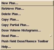
The “Plans” pull down is on the main menu. Options that do not belong to the Dosimetry Check function but that might otherwise be part of general treatment planning are either grayed out or do not appear. The Dosimetry Check plans are saved under the selected patient directory in a separate subdirectory ckpn.d.

Under the Plans pull down menu are options to create a new plan, to retrieve an existing plan, to edit an existing plan, to copy a plan, or to delete a plan. When a plan is retrieved, the name of the plan will be added to the bottom of pull down for quickly assessing the plan again from the main toolbar.

The “Copy Plan” function copies the entire plan. The “Copy Partial Plan” function does not copy the fluence files or dose matrices that were created from computing the dose, leaving the copied plan in a state that cannot be computed until fluence files are read in for the beams.

If you have downloaded the plan, the beam’s should be set to the proper location in the stacked image set and angles. Otherwise you will have to locate isocenter and type in the gantry, couch, and collimator angle for each beam that you create. The plans and beam parameters are saved as you create and change them. Some beam parameters are saved when you return from the beam’s toolbar. Dose matrices are saved when you return from the plan toolbar.

Note that you may select or create more than one plan, and may selectively display each plan in different frames.

As you retrieve or create plans, the plan name will be added to the bottom of the pull down for quick access from the Plans pull down.

Dose Volume Histograms

You can compute the dose volume histogram for outlined regions of interest. The dose is that computed by DosimetryCheck, not by the other treatment planning system. Shown below is the volume histogram popup. We will refer you to the RtDosePlan manual for details on the use of this option, under the Plan section. Dose volume histograms are provided here as there may be some use in comparing to the planning system. In summary, you can select the same volume for different plans, as well as different volumes. Hitting the compute button will start the computation which you can stop when the plotted curves have settle down.

While the computation is running more points are being computed. When any volume reaches a point to volume density of 1000 (1000 points per cc) that volume will not be computed anymore. The computation will stop if all volumes reach that density.

See: Andrzej Niermierko and Michael Goitein, "Random Sampling for Evaluating Treatment Plans," Medical Physics, 17(5), Sep/Oct 1990, pages 753-762.

We simply continue to generate points at random until either the stop button is hit or all selected volumes reach a density of 1000 points per cc.

Note that you can select to view the accumulated volume histogram in terms of cc or % of volume. Also you can toggle the background between white or black.

The dose volume histogram can also be recomputed and displayed from the downloaded 3D dose matrix from the planning system (called the TPS or Foreign dose) and shown as a dotted line.

You also have access to this control from the Evaluate pull down on the Plan toolbar.

Dose Volume Histogram

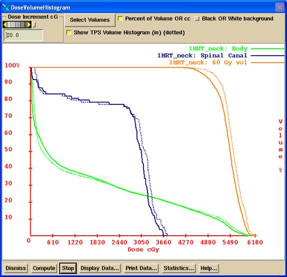
The “Display Data” button will print the data to a file and then display the contents of the file, which may be suitable to imputing to some other analysis tool, or you can print from there. The statistics button will compute the minimum and maximum dose, the average dose, and the standard deviation of the dose to each volume, for both the reconstructed dose and the plan dose.

Dose Volume Histogram Statistics and Dose Volume Limits

Dose statistics such as the minimum dose, maximum dose, and average dose to a selected ROI volumes are computed and displayed in the Statistics. An example is shown below:

Min Dose Max Dose Ave Dose Standard Volume

cGy cGy cGy Deviation cc

Plan: IMRT_Neck

DC Reconstructed (5910 points):

PTV 3766.2 6221.2 5560.1 5.7% 1258.7

Reference TPS (5910 points):

PTV 2678.3 6217.6 5551.9 4.7% 1258.7

DC Reconstructed (32614 points):

Body 0.0 6220.2 1642.0 121.6% 13819.9

Reference TPS (30931 points):

Body 0.0 6271.4 1650.6 109.3% 13819.9

DC Reconstructed (2011 points):

esophagus 3663.3 5314.7 4511.4 4.3% 9.7

Reference TPS (2011 points):

esophagus 3017.6 5211.8 4507.7 6.2% 9.7

In addition, pass fail for dose volume limits are computed here as described below (starting with version 5 release 7). An example is shown below (dose limit values are made up bogus numbers for illustration):

TARGET PTV

Minimum average permitted dose 5600.0cGy

DC number points 5951 average dose 5559.3 fail

TPS number points 5951 average dose 5551.4 fail

Minimum permitted dose 2500.0cGy

DC number points 5951 minimum dose 3381.8 pass

TPS number points 5951 minimum dose 2678.3 pass

Maximum permitted dose 6200.0 cGy

DC number points 5951 maximum dose 6221.2 fail

TPS number points 5951 maximum dose 6217.6 fail

Maximum permitted fraction 0.5000 for dose under 5500.0cGy

DC number points 5951 fraction 0.3685 pass

TPS number points 5951 fraction 0.4211 pass

ORGAN_AT_RISK esophagus

Maximum permitted dose 5500.0cGy to the entire volume

DC number points 2011 minimum dose 3663.3 pass

TPS number points 2011 minimum dose 3017.6 pass

Maximum permitted dose 6000.0cGy to any part

DC number points 2011 maximum dose 5314.7 pass

TPS number points 2011 maximum dose 5211.8 pass

Maximum permitted fraction 0.1000 for dose over 5000.0cGy

DC number points 2011 fraction 0.0159 pass

TPS number points 2011 fraction 0.0179 pass

See also the webpage summary later below.

Volume Histogram Dose Limits

Version 5 Release 7 of DosimetryCheck introduced this new feature. The plan can be evaluated in terms of the dose volume histogram in regards to stated goals of the treatment plan, such as maximum and minimum dose and other specifications outlined below. A volume histogram dose limits protocol file must have been selected for testing if a plan meets the dose volume specifications. There are three ways to specify the dose limits to be tested:

(1) If the protocol was included in the treatment planning system structures and plan Dicom RT files that were imported, then you do not have to do anything as the limits will be picked up from the download (however Dicom does not include the maximum average dose to an organ at risk or the minimum average dose to the target).

(2) If you have protocol files and if the name of your plan matches the name of the protocol file (for example plan name is prostate and there is a protocol file named prostate or prostate.txt), then that protocol file will have been copied already to the plan folder. The name match will be case insensitive.

(3) You can select a protocol file in program ReadDicomCheck for the plan after importing the plan file.

(4) You can select a protocol file from Dosmetry Check under the Options pull down on the Plan toolbar.

If the volume specifications came from the Dicom download, the file is saved with the name DoseReferenceVolumes.txt. If a protocol file is copied in, that file is saved with the name VolumeDoseLimits.txt. The program will first look for the file VolumeDoseLimits.txt and only if it is not there will it look for the file DoseReferenceVolumes.txt when computing pass fail. Hence VolumeDoseLimits.txt has precedent but that gotten from the Dicom download is preserved.

The volume names in the stacked images set must be identical to the names in the protocol files. Note that Dosimetry Check will strip out all characters which cannot be in a directory (or file) name because each ROI volume is stored with the name as a folder name, and replaces spaces with an underscore. The list of volume names will be added to the list in the Auto Report for dose volume histograms if a matching name is found. The pass fail is reported in the statistics section of the dose volume histogram (above) and so that must be chosen in the auto report (see AutoReport below). See also the log summary presented in a web page below.

The protocol files are stored in the folder:

c:\mathresolutions\data.d\VolumeDoseLimitProtocols.d

where data.d is in whatever folder the Dosimetry Check executables were installed in. The user must write or provide the protocol files, the format is described below.

The two files DoseReferenceVolumes.txt and VolumeDoseLimits.txt are editable but normally one will select a different protocol file to make a change. To turn off computation of dose limits just select a protocol file with empty entries. The selected file is stored in the plan folder:

folder_of_patients\patient_name_number\ckpn.d\plan_name

where the location of folder_of_patients is defined by the program resource (preference) file “PatientDirectory.loc” which is in the program resources folder, which in turn is defined by the file “rlresources.dir.loc” in c:\mathresolutions (or what ever is the current directory).

ROI volumes constructed from contours

The Dicom standard covers how contours are transferred, not how volumes are created out of those contours. Therefore, there may be small differences between the volumes computed by Dosimetry Check (System 2100) and those by the planning system. Dosimetry Check formats the volume in terms of a three dimensional matrix of three dimensional square voxels. A voxel is either inside the volume or not. The size of the voxel will have some affect. The surface generated for display is by means of the marching cubes algorithm and is not used for determining the boundaries of the volume.

Whether a voxel that a contour goes through is considered inside or outside the volume might differ. Dosimetry Check by default does shape interpolation between the planes of contours every mm (the user can turn that off, see “Outlining Regions of Interest” in the System 2100 reference manual). A CT scan is considered to define the space halfway to the next CT scan (but pixels are interpolated between parallel scans in reformatted images). Not an issue here, but Dosimetry Check can also incorporate contours made in reformatted images. This appears to not be an issue because three dimensional contours are not supported by other planning systems.

The dose volume histogram reported for the planning system is computed for the same points generated by Dosimetry Check using the three dimensional dose matrix from the planning system. The dose volume histogram from the planning system is not imported.

Dicom RT Volume Dose Limits

The Dicom specifications are described here and are for volumes, not points. The Dicom specified dose volume attributes are the tags (300A, 25 to 28) for targets and (300A, 2A to 2D) for organs at risk. There are three specified limits for target and three for organ at risk:

Dicom (300A, 25) the minimum dose limit to a target. No point in the target may get less than this dose.

Dicom (300A, 27) the maximum dose limit to target. No point in the target may get more than this dose.

Dicom (300A, 28) the maximum fraction of the target that can get less of the prescribed dose specified in Dicom (300A, 26).

And for organ at risk:

Dicom (300A, 2A) the maximum dose the entire organ can receive. Our interpretation is that the minimum dose to the organ cannot be more than this dose.

Dicom (300A, 2B) the maximum dose any part of the organ can get.

Dicom (300A, 2D) the maximum fraction permitted to get a dose more than that specified in Dicom (300A, 2C).

In addition we have added a test for the average dose limit to a target, the average dose may not be less than this dose. And we have added a test for the average dose limit to an organ at risk, the average dose may not be more than this dose. A protocol file would have to be written to include these last two added items.

Volume Dose Limits Protocol File

An example protocol file is shown below. Be advised that the actual numbers below are totally bogus and were made up for this example and have no clinical relevance. The file format is under the ASC text file standard defined in the System 2100 reference manual in the “Program Resource Files” section. Briefly, white space separates items to be read. Anything from /* to */ is not read and anything after // to the end of the line is not read, and constitutes comments. In this manner the file can be self documented with the use of the above comments.

The file format begins with an integer 1 which defines the format version of the file. If additional specifications are added in the future, the format version would be boosted to 2 so that a new program can read an older file.

For each ROI volume is expected two text strings followed by 5 numbers.

The first text string must be “TARGET” or “ORGAN_AT_RISK”. Targets and organs at risk can be in any order in the file.

The second text string must be the name of the ROI volume. This text string should be incased between <* and *> so that a space in the name will not be taken as white space that would otherwise separate items to be read. The name must exactly match the name of an ROI volume and the comparison is also case sensitive. Prostate will be different from prostate. A review of the names presented in Dosimetry Check should be made as characters not permitted in a folder name are stripped out and spaces are replaced with an underscore with no more than one space permitted between characters.

The five numbers that must follow meaning will depend upon whether the item is a target or an organ at risk. Any number may be replaced with a -1 to designate that the limit is not specified and a report on pass fail will then not occur for that specification.

For a target the numbers are to be, in order:

Dicom (300A,25) The minimum permitted dose.
Dicom(300A,27) The maximum permitted dose.
Dicom(300A,26) The prescribed dose for the below fraction.
Dicom(300A,28) The maximum permitted fraction to get less than the above dose in (300A,26).
The minimum average dose.

For an organ at risk the numbers are to be, in order:

Dicom (300A,2A) The maximum permitted dose to the entire volume.
Dicom(300A,2B) The maximum permitted dose to any part.
Dicom(300A,2C) The dose for the below fraction.
Dicom(300A,2D) The maximum permitted fraction to get more than the above dose in (300A,2C).
The maximum average dose.

There may be 0 to any number of targets. There may be 0 to any number of organs at risk. The example file is:

/* file format version: */ 1

// an entry of -1 means a valid number not provided

//TARGET cGy

// Dicom(300A,25) Dicom(300A,27) Dicom(300A,26) Dicom(300A,28)

// Minimum Dose Maximum Dose Prescription Max UnderFraction

// Minimum average dose

TARGET <*PTV*> 5800 6500 6000 0.20 6000

TARGET <*SecondaryTarget*> 2500 6200 5500 -1 -1

//ORGAN_AT_RISK cGy

// Dicom(300A,2A) Dicom(300A,2B) Dicom(300A,2C) Dicom(300A,2D

//Maximum Full Dose Maximum Part Dose Maximum Risk Dose MaxOverFraction

// Maximum average dose

ORGAN_AT_RISK <*esophagus*> 5500 6000 5000 0.10 -1

ORGAN_AT_RISK <*SpinalCanal*> 4000 4500 3500 0.10 3000

The following would also be a correctly formatted file as the above comments are ignored, and only white space is needed to separate items:

1 TARGET <*PTV*> 5800

6500 6000 0.20 6000

ORGAN_AT_RISK <*SpinalCord*> 4000 4500 3500 0.2 3000

ORGAN_AT_RISK <*kidney*> -1 3500 -1 -1 -1

Use the template file provide in folder data.d\VolumeDoseLimitProtocols.d to write a protocol file.

Volume pass fail log web page

The Auto Report will write a summary to a log file. The location of the log file is defined by the program resource file “PatientVolumeAutoReportLog.loc” in the program resources directory (defined by the file rlresources.dir.loc in the current directory). The contents of the file is:

/* file format version */ 1

// path to the folder where the patient report log file is to go

// for report on volumes pass and fail.

<*g:/PatientLogReport.d*>

The user must decide where the folder for the log is to go. The log file will have the name “PatientVolumeLog.htm”. The log file is a webpage to be looked at by any web browser. The user must type in the URL of the webpage. For the above example it would be:

File:///g:/PatientLogReport.d/ PatientVolumeLog.htm

This URL can be saved as a book mark for convenience. Be aware that if the web browser is caching viewed web pages, the user might have to hit the reload button to see the latest version of this file rather then the prior cached copy. The page will show a summary of the results of the AutoReport for the volume dose limits, and provide a link to the Auto Report. An example of the summery web page PatientVolumeLog.htm is shown below:

Doe_John_1234 Plan: IMRT_Neck Date: 08-Mar-2018-21:15:59(hr:min:sec)
2 Targets, 3 organs at risk
All Target 8 FAILS for DC. All Organ 10 FAILS for DC.
All Target 8 FAILS for TPS. All Organ 10 FAILS for TPS.
Auto Report

Doe_John_1234 Plan: IMRT_Neck Date: 08-Mar-2018-21:21:01(hr:min:sec)
2 Targets, 3 Organs At Risk.
All Target 8 PASSES for DC. All Organ 10 PASSES for DC.
All Target 8 PASSES for TPS. All Organ 10 PASSES for TPS.
Auto Report

Doe_John_1234 Plan: IMRT_Neck Date: 08-Mar-2018-21:24:53(hr:min:sec)
2 Targets, 3 Organs At Risk.
CAUTION Target for DC: 3 passes, 3 fails. CAUTION Organ for DC: 6 passes, 3 fails.
CAUTION Target for TPS: 3 passes, 3 fails. CAUTION Organ for TPS: 5 passes, 4 fails.
Auto Report

If this file gets too long, the user can delete it and a new file will be created the next time the program needs to write to it.

Plan Toolbar

The Plan Toolbar.

Once you have selected or created a plan, the plan toolbar will be displayed. When the plan is first created you will be required to select the primary stacked image set. This set will specify the skin boundary and the pixel to density conversion curve. Once you have selected the primary image set, you cannot change it. Under those circumstances, you would have to delete the plan and create a new one. The toolbar shows the current plan name in an option menu. You may select different plans with this option menu among the plans that were currently retrieved or created with this run of the program. Next on the toolbar is the name of the primary stacked image set once it is selected, or an option menu to do so if not yet selected.

If you downloaded the plan using the RTOG or Dicom RT protocol, the stacked image set will have been determined. However, neither protocol specifies CT number to density conversion, and so you must select that. Go to the main toolbar to Options under the Stacked Image Set pull down. Then select Density and select a curve. The Dicom RT protocol can specify which ROI volume is the skin boundary, but the RTOG protocol does not. So if the RTOG protocol was used, you will also have to select which ROI volume is the skin boundary. Select Skin on the same Stacked Image Set Options toolbar and select the skin boundary ROI with the option menu provided. If a skin boundary was not downloaded, you can use the automatic skin boundary generation tool on the contouring toolbar. See the System2100 manual, contouring section.

Dosimetry Check will then attempt to find field dose files for each beam that does not have one. The program will look for files that include the beam name in the file name. All such files found for a particular beam will be added together. The directory searched is the FieldDose.d directory in the patient’s directory where program such as ConvertEPIDImages places files after calibration and deconvolution. The plan name and beam name will be shown on each field dose image. The files used to create the field dose will also be shown if there is room. Maximize the frame to see all the text.

Beams Pull down

The Beams pull down menu has to do with creating and editing beams that belong to the plan. You can create, edit, and delete beams. When you create a new beam it will start out with the isocenter of any prior beam in the same plan if not the first beam. You can also create a new beam that has the same isocenter and angles of a prior existing beam, or create a new beam that is to be parallel opposed to an existing beam. From this pull down you can select a beam to have all the other beams to have the same isocenter location. Each beam is stored in a subdirectory under the plan’s subdirectory.

For the Dosimetry Check program, only x-ray beams may be selected. We presently do not support electron beams with this function. Most electron fields are applied at a fixed distance and the monitor units applied is close to the dose delivered, and so the quality control problem is not so involved as it may be for x-rays.

Display Pull down

Under the Display pull down are options pertaining to displaying the plan. Because there may be more than one plan in the run of a program, the plans are not automatically displayed in frames. Rather you must select which frames to display the plans in. You can specify a specific frame on all the frames on the currently displayed screen. However, the program will not allow a plan to be displayed on an image that does not belong to either the primary stacked image set or on an image set not fused to the primary image set. A plan cannot be displayed in a frame in which a plan is all ready displayed. What is displayed are the beams, point doses, and isodose curves if also selected for display.

Display Plan Control Popup.

A popup tool is provided to remove a plan from being displayed in a frame. The same controls appear to display a plan but additional controls are provided to remove a plan from a frame or screen.

Controls for turning off and on beam displays is provided. The central ray is drawn as a solid line to isocenter, and then drawn as a dashed line beyond. The beam’s eye view x, y, and z axes are drawn and marked. The z axis is the central ray, positive toward the source of x-rays, and lies coincident with the central ray. With the treatment machine pointed at the floor and the collimator unrotated, the x axis goes from left to right while standing in front of the treatment couch looking toward the gantry. The y axis is parallel to the long axis of the unrotated treatment couch and points toward the gantry. The origin is at isocenter. The Dosimetry Check program has not have the concept of field size since the field is defined by a measured picture of the x-ray field (even though the field collimator positions are defined in the field image data structure).

You can select a default display of transverse, coronal, sagittal, and 3D room perspective view centered on the CT data set, a particular outlined region of interest, a particular point, or the isocenter of a beam. Normally, however, one would pick image planes to correspond to that shown on the planning system. The reformat image option under the Stacked Image Set pull down on the main toolbar would be useful for this purpose.

Calculate Pull down

Items under the calculate pull down have to do with calculating the dose. Because calculation times may be long, there is control to selectively select which frames the dose is to be displayed in. Each frame is calculated when it is selected here to display the dose. The hot spot in that frame will be displayed and marked with a star asterisk like figure. You can also select to compute all beams in the entire patient volume to get that done before evaluating the dose.

Dose Matrix

Each beam maintains a dose matrix on diverging fan lines, the fan lines covering the area of the beam. A rotating beam would be simulated with multiple dose matrices at increments specified by the plan. The spacing between the fan lines and along the fan lines is also specified by the plan, so that all the beams belonging to a plan use the same parameters. Each beam stores its matrix under its own subdirectory under the plan subdirectory. The matrices are written to disk files when the return button on the plan toolbar is activated.

For any two dimensional plane image displayed in a frame a two dimensional matrix will be generated that covers the entire image. The same spacing parameter specifies the distance between points. When the dose is calculated, the coordinates of each node of the two dimensional matrix is passed to each beam. The beam module will find the diverging box bounded by the fan lines that the point is inside. The eight corners of the box will be referred to when interpolating the dose at the position of the passed in point. Each beam will calculate the dose to each vertex of the diverging box on a need basis: “compute on demand”. When ever a reference is made to a vertex where the dose has yet to be computed, the dose is computed at that time. After calculating the dose to a plane, all the beams will have a swath through their dose matrices of calculated points. As more planes are computed, more of each beam’s dose matrix is computed. If any change is made to a particular beam, that beam’s matrix is reinitialized.

Likewise when a dose in a 3d perspective room view is computed, a rectangular array (lattice) of points is generated for the patient volume. Each of those points is likewise passed to each beam, so that after a room view display each beam will most likely have calculated the dose to all of the available vertices.

Calculate All Beams 3D

The Calculate All Beams 3D option will force all the beams to compute the dose to all the vertices on their respective dose matrices.

Parallel Processing

For releases on and after Sept 20, 2012, parallel processing is supported. The number of threads that an instance of program can create is to be specified in the file NumberOfThreads.txt in the program resources directory. An example file is:

/* file format version: */ 1

// The maximum number of threads a program is to create

// for parallel processing. This should be the number

// of hardware threads (we suggest setting one less).

// A value of 1 or less will turn off parallel processing

You will gain nothing in performance in setting more threads than there are hardware threads on the computer. An I7 has a total of 8, hence 7 above is set in the file (7 in addition to the main thread is 8). A value of 1 or less will disable parallel processing. Multiple instances of the program are not considered in the number of threads that an instance will create.

Any requirement for the dose in the entire patient volume will also trigger the calculation of the entire patient volume for all active beams and will allow the use of parallel processing. This will occur when gamma analysis is invoked, dose volume histograms, dose difference volume histograms, selection of the auto report, or display of dose in 3D. If you are first looking at profiles or isodose curves, you might want to make this selection to compute the dose up front for all beams in parallel which might over all be faster than waiting for the on demand computation as described above.

Calculation Matrix Spacing and Rotation Increment

Calculation Matrix Spacing Control Popup

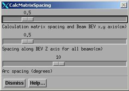
A control is available to specify the spacing to use for all the dose matrices and the increment in rotation to simulate beam arcs. Making a change here will force all beams to dump their current dose matrices. The matrices covering planes and the matrix for room views also must be regenerated if a change in spacing is made here. The user will then have to reselect the frame to display the dose in.

The calculation matrix spacing is the distance between points on two dimensional images and between the three dimensional dose matrix. Each beam is queried for a value at these points. Each beam maintains its own divergent matrix within which points are interpolated. The calculation matrix spacing is used in the plane perpendicular to the central ray in the center of the patient. The spacing along the BEV Z axis is the spacing parallel to the central ray. You might want to use a smaller calculation matrix but leave the spacing larger as there is less of a gradient along the diverging rays.

The arc spacing is the increment to use to simulate an arc with fixed beams. This parameter is adjusted somewhat by each beam to fit the arc length of that beam so that the arc is simulated with equally spaced fixed beams.

Default Matrix Spacing

The matrix spacing can have default values specified in the file DefaultCalculationMatrixSpacing.txt in the program resources directory. A sample file is shown below:

/* file format version */ 1

// file to specify the default matrix spacing for calculation of dose

// spacing in the plane perpendicular to the central axis in cm

// minimum 0.1 cm, maximum 2 cm

0.5

// spacing along the diverging rays in cm

// minimum 0.2 cm, maximum 2 cm

0.5

// for rotating beams with fixed field shape or fluence file

// increment to simulate a rotating beam in degrees (integer only)

// minimum 1, maximum 20

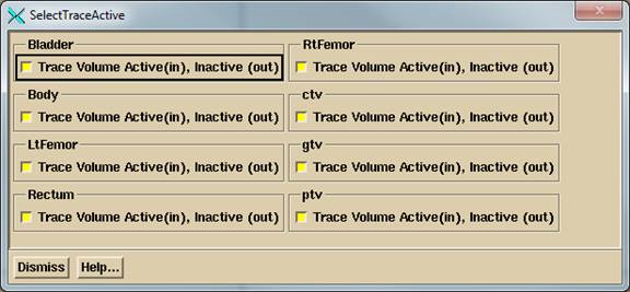
ROI Volume Trace Control

All the ROI volumes are considered collectively when tracing through the stacked image set. If for some reason you do not want an ROI volume to be considered, you can turn off that volume for this purpose. You might want to do this if you have a volume that sticks outside of the patient skin surface but do not want that protrusion to be considered. Be aware that if part of the volume is inside some other volume that is on for this purpose, then the ray will still be traced through that part of the volume that is inside the other volume. This does not turn off any assigned density to the volume. Do not turn off the skin surface volume, otherwise your calculation might not consider the patient model.

An example of the pop up tool is shown below. The area will become scrolled for a large number of ROI volumes.

Specific Points

At this writing, the plan does not have its own list of specific points. Rather, the only list of specific points is maintained by the primary stacked image set. Therefore all plans using the same stacked image set will calculate the dose to the same list of specific points. The controls for the specific points are under the Stacked Image Sets pull down on the main toolbar. Select Options and then Points.

However, we need the ability to specify the coordinates of a point in terms of the beam’s eye view coordinates of a specific beam or the IEC image set coordinates relative to isocenter. Therefore a control is provided here for adding a point where the position is known relative to isocenter. The coordinates are then transformed to the stacked image set coordinates and the point is created and saved. The point is not moved if the beam is later moved. To delete a point use the above controls for points as described under the Stacked Image Sets Options.

Plan Points Toolbar.

Under the Evaluate pull down we have a points toolbar. Here the dose to the specific points may be computed, displayed, printed, or saved to a temporary file. We can select the popup to enter new points in beam’s eye view coordinates or IEC couch coordinates relative to isocenter. There is also a mechanism for comparing measured to computed values for testing purposes.

Print Points

Simply hitting this button will cause the points to be computed and printed. The plan dose will also be printed if the point falls within the 3D dose matrix gotten from the planning system.

File Points

Selecting this option, the point’s label and dose value will be written to a file in the temporary file directory where print jobs are also stored. The dose to the points are first computed. An example file follows:

// Test Square 12-Dec-2000-09:19:19(hr:min:sec)

// Label Dose in cGray

<* Example Label *> 1.299286

<* slice 10 row 4 column 7 *> 1.324436

The file is written in our ASCII standard whereby comment lines start with two slashes and are not read. The label for the point is enclosed between the <* and *> symbols. The dose value is simply a number set off by white space. This format will also be referred to below.

Display Point Doses

This choice will display the dose value computed for each point below the label for the point in all frames where the plan is displayed. The planning system dose, if available, will be interpolated from the TPS 3D dose matrix with the letter P preceding the value displayed. There is also a button on the Evaluate pull down on the Plan toolbar to do the same thing.

Point Dose Off

This will turn off the display of the dose value of the points. Note also that any change to the plan or a beam will also turn of the display of the dose values.

Add Point In IEC

Locate Points in BEV or IEC Image Set Coordinates Control

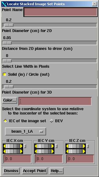
This tool is provided here as a convenience so that a point can be added to the stacked image set in reference to the beam’s eye view coordinates of a beam or the image set relative to isocenter. The control is very much like the one provided by the stacked image set under Options to Points toolbar. However, we have added an option menu to select the beam to define isocenter and two radio buttons to select the coordinate system to use.

Below the option menu are controls for the x, y, and z coordinates of the point. The point may not be located with the mouse here. Do that on the control provided by the stacked image set under the Stacked Image Set pull down on the main toolbar, to Options. The control provided here is for the case when a point must be specified in relationship to isocenter in the coordinate system of a beam or an IEC system relative to isocenter and the image set.

The beam’s eye view coordinate system is described elsewhere as well, where in the unrotated collimator and gantry positions (beam pointed at floor), the x axis goes across the couch left to right when looking into the gantry, the y axis points toward the gantry along the gantry’s axis of rotation, and the z axis points toward the source of x-rays. The x and y axes rotate with the collimator in BEV and the show system rotates with the gantry. The origin is at isocenter.

The IEC image set system is fixed to the patient. The Y+ axis in the image set is always towards the patient’s head. The Z+ axis is always up. The X+ axis is to the patient’s left for a supine patient, right for a prone patient. Here the origin is at the isocenter of the selected beam.

To delete or otherwise edit points, use the other controls provided by the Stacked Image

Set Options.

Compare to Measured

This option was provided for a very narrow purpose. Specifically, we irradiated a Rando Phantom and measured the dose at specific points and wanted to be able to display the measured value with the computed value. The measured values must be written to a file in the same format as the computed points are written to as described above. Selection of this option will prompt you to enter the file name of the measured points. The measured points are associated with the computed points by means of the point’s label. The labels are not directly compared. First each label is converted to lower case and then all spaces are removed and then compared. Care must be taken that the labels will remain unique when the user creates the labels. For a match, the measured value will be displayed below the computed value. An m is also appended to the measured dose value. In our use of the Rando Phantom we labeled the holes according to a scheme. There are 7 rows and 13 columns of holes with the 3 cm matrix drilling. Each hole is known by its slice number, row number, and column number. By labeling the holes consistently, the measured values can be matched up with the computed values and displayed. The specific points are also computed upon selecting this option.

We have also written a program that will compare measured and computed values, CompareRandoPoints. Invoke this program and on the command line provide the name of the file that contains the measured points, the name of the file that contains the computed points, and the name of a file to write the report to. This program assumes that only numbers appear in the label field, consisting of the slice number, row number, and column number separated by spaces and sorts values by those indices.

This labeling scheme could cause some confusion in the above display function in frames as 11 1 1 would be indistinguishable from 1 1 11, for example, after removing spaces. The row number is only in the range of 1 to 7 and the column goes only from 1 to 13. Use leading zeros for the slice number and column number for single digits if there is a possibility of confusion, i.e. 11, 1 01 and 01 1 11.

Selection of Algorithm

The selection of the algorithm to use may be selected here under the calculate pull down:

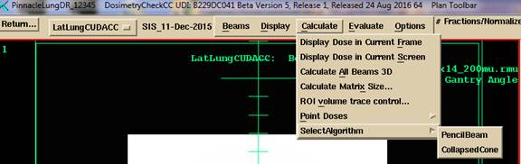
Note however, that the algorithm will in general default to the designated source of the Sp factors used to compute the Sc factors used to fit the EPID deconvolution kernel. See the section in the algorithm section titled “Collimator in-air scatter factors”. The source of the Sc factors is tracked from the EPID deconvolution kernel to the rmu file that is produced. The program will default to the algorithm used for the source of the Sc factors unless over ridden here.

For the convolution/superposition “collapsed cone” algorithm, there is an option to specify the number of azimuth angles from 8 to 36. The published journal paper: “A nonvoxel-based dose convolution/superposition algorithm optimized for scalable GPU architectures”, Medical Physics Vol 41 No 10, October 2014, pages 101711-1 to 101711-15, on page 11 stated that “The accuracy study presented above showed that an angular sampling combination of 8x8 produced acceptable results”. Their “ground truth” was a computation with 48 x 48 rays (cones). The number of zenithal angles is here fixed at 8 (22.5 degrees spacing, 0 to 180 degrees). The default is 18 azimuth angles for Version 6 release 6 (20 degrees spacing from 0 to 360) if this file does not exist. We have not noticed a significant difference in accuracy from 18 but we have seen differences of the order of 2%. You may specify your choice in the file DefaultDoseAlgorithm.txt in the program resources folder. See the Dose Algorithm section of the manual for more details. This file will govern the number of azimuth angles when ever the collapsed cone algorithm is used. This file will default the algorithm choice for TomoTherapy.

Evaluate Pulldown

Items under the evaluate pull down have to do with displaying the result of calculation. See below for the options under Hard Copy.

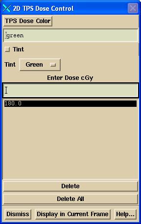
Two Dimensional Isodose Control

2d Isodose Control

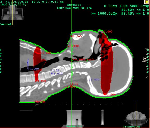
This control provides a tool for the user to specify the isodose value to be displayed. For the Dosimetry Check function, only the dose may be displayed in cG. The dose value desired is to be typed in the text field at the top of the popup. The line width may be changed to make a particular isodose line stand out. The isodose value may be tinted in a single color showing the boundaries and interior (higher doses) of that isodose line. You may use the mouse to select different isodose values to tint on the scrolled list below the text field for the value entry. Note also that the tint may be turned off and the tint color may be changed among the primary colors and additions of any two of the primary colors. Likewise any selected isodose line may be deleted or have its color changed. Colors are initially assigned at random. Note also that each isodose line has tick marks on the down hill side (lower dose) of the isodose line, analogous to topographical maps. The selected isodose lines apply to all 2d frames in which the dose has been selected to be displayed for the plan.

An issue that must be dealt with is what to do when two successive dose vertices span the skin boundary, so that one point is outside the patient and the next point is inside the patient. The plotting of the isodose line simply stops at that point. However, the tinted area necessarily requires a closed contour.

Warning, tinted dose near skin surface:

In those regions the tint follows a path between points inside the patient and outside the patient and does not accurately represent the dose.

Three Dimensional Isodose Control

3d Isodose Control Popup.

A three dimensional isodose surface may be shown in 3d perspective room views of the primary stacked image set or any image set fused to it. Only one surface can be shown at a time. The desired value is typed into the text field provided. Under the text field is a control for the transparency of the isodose surface.

Limitations apply here. A transparent surface can only be seen inside a second transparent surface if the inside transparent surface is drawn first. Two transparent surfaces that intersect will present a problem in that if surface A is drawn first and surface B is drawn second, then surface A can be seen inside surface B, but surface B cannot be seen inside surface A. This software will draw the transparent isodose surface before other transparent surfaces. No attempt is make to sort surfaces or part of surfaces. If this becomes a problem you have two options. One, make all the other surfaces opaque or make the isodose surface opaque. You can also use a cutting plane on volumes that are drawn. A second option is to display the isodose surface in wire frame. The wire, solid, off, control is below the transparency scale.

This control controls all frames simultaneously that show 3d room perspective views where the user has chosen to show the dose. The user must first choose to display the plan in the frame.

Dose Comparison Tools

Several tools are provided for comparing and showing the dose distribution that may have been downloaded from the treatment planning system. These tools can be used for enhancing your understanding of any dose difference. The tools are found under the Evaluate pull down.

Display Point Doses

See this option on the Plan Points Toolbar above.

Show Point Dose Values

You can click the mouse on images and get the computed Dosimetry Check (DC) and Treatment Planning System (TPS) plan (also called foreign) dose.

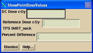
To display the percent difference, you must first enter a normalization dose for the gamma method on the gamma method control (or Auto-Report, both below). The percent is computed relative to that value. The percent difference between two values is not shown here. If the prescription/normalization dose is 200 cGy, and in some low dose area there is a computed dose of 11 cGy versus a plan dose of 10 cGy, then the percent difference is ½ percent, not 10 percent.

Compare 1D Dose Profile

You can compare the dose profile between the planning system and reconstructed dose for any line through the patient space. Do you this by selecting any reformatted image through the patient, and then positioning a line on that plane. Shown below is an example. You first must select a current frame. The current frame must be showing a plane through the stacked image set of the plan or one fused. Use the reformat image control to select different planes through the patient (under the Stacked Image Set pull down on the main tool bar). Then use the translate and rotate controls to position the line visually. Hit the “Get Profile” button to see the curve. If you do anything that changes the dose, you must hit the “Get Profile” button again to update the displayed data.

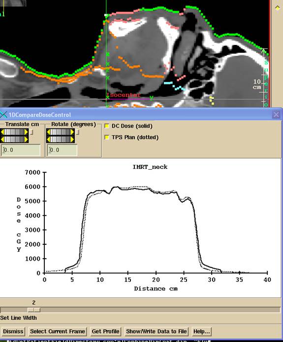
The Show/Write Data to File button will display the data that is plotted and write to an ASCII file.

Compare 1D Dose Profile Relative to a Beam

There is another similar control that will allow you to specify a profile relative to a selected beam in beam’s eye view coordinates (BEV). Here you will select the beam from a cascade on the Evaluate pull down. You will then select the Z BEV coordinate for the profile and an angle of the profile, rotated around the Z axis from the X axis. Isocenter is at Z = 0, and points further away from the source are negative.

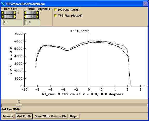
Nothing is drawn on images on the main window. In the above example, the profile is shown along the BEV axis for beam “A3 rao” through isocenter (since BEV Z is zero and the rotation angle is 0). The dose is still shown for all beams however. If you want to compare the dose for only one beam, you will have to download a plan for only beam.

Compare 2D Isodose Curves

You can select to view isodose curves together from the downloaded TPS dose along with the dose computed here. Or show one or the other, or show the difference between the two dose sets. The dose difference is the absolute value between the DC computed and TPS dose. The TPS dose distribution (and so also the difference) will be limited by the area covered by the read in dose array. Isodose curves will not be plotted outside that area nor outside the patient surface. By necessity the tint must be a closed area and so may have to follow along the skin surface. Where the corresponding isodose curve is not plotted, the tint boundary cannot be taken as accurate but only approximate.

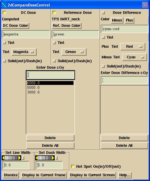
2D compare dose control

Hit the "Display in Current Frame" button to display the dose in a current frame that contains an image from the primary image set or one fused to it. Hit “Display in Current Screen” to display in all the frames on the currently selected screen. This will not engage any particular frame however. If a 3D calculation has not been done, all frames in which the dose can be shown on the screen will be calculated and could take some time. You might want to consider reformatting a stacked image set on the main tool bar for a smaller set of images other than the entire stacked image set.

On the top row you can select which dose you want to see:

DC Dose: that computed here.

TPS Plan: that read from the other planning system.

Difference: the difference between the two.

You can select any combination of the above to display.

Below that, you can select the color the isodose curves are displayed in and the tint color. ONLY ONE of the three sets may have a value tinted in, and only a single selected value will be tinted. The tinted area is for the dose or greater. See also the note above about the tint area along the skin boundary. Select a dose value with the mouse to select the value to be tinted. For dose difference, doses smaller then the plan dose (minus) are shown in a different color from doses larger than the plan dose (plus).

Each set of isodose curves is shown in the same color, so that it will be easy to distinguish which curve belongs to which set. The SAME values are displayed for the DC computed and TPS doses. You can specify a separate value for the dose difference. You can select a dashed line for any of the three sets of isodose lines (Dosimetry Check result, the planning system, or the dose difference) with the corresponding toggle button. The line width sets the width for all three sets of isodose lines. The dash length sets the dash length for any dash that is selected.

Use the delete button to delete any currently selected isodose value. Use the delete all button to delete all the values from the respective list.

Note that the hot spot for each data set will be displayed in the same color as the isodose lines are drawn in. Hot spot is displayed with an ‘*” and can be turned off or on.

This control will disengage from the display if a different frame is selected as the current frame. Hit the "Display in Current Frame" button to reselect the frame or a different one.

Any color changes you make will be saved and also used as the default for new cases.

Compare Dose in 3d Room View

To engage this control with a current frame, you must first make a 3d room perspective view of the primary image set of the current plan or an image set fused to the primary image set. Use the "Screen Control" button to create a new screen if need be, and select an empty frame by clicking the mouse on the button covering an empty frame. Then go under "Stacked Image Sets" on the main menu to "Display Room View".

Compare 3d Dose Control

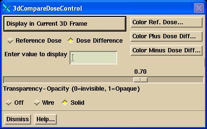
Select "TPS" or "Dose Difference", then hit the "Display in Current 3D Frame" button. This control will disengage from the current frame if you reselect the "TPS" or "Dose Difference" buttons, or if the frame is no longer current or visible. To reengage, simply hit the "Display TPS Dose in Current Frame" button again. You may also select a different frame any time, with multiple frames showing the same or different display and dose values.

Selection of "TPS Dose" will simply show the dose from the other system. "Dose Difference" will show the absolute value of the difference in dose between the other system and that computed here. Positive differences are shown in a different color than negative differences. The default for positive differences is red and for negative is cyan.

Type in the dose or dose different value to display in the provided text field, hitting the Entry key at the end of the number string. You can also change the transparency of the isodose cloud, and select wire frame instead of solid, as well as turn off the cloud display.

Lastly, you can change the color of the cloud for either the TPS dose, or the positive or negative difference.

Gamma Method

The gamma method is a method to compare two dose distributions. The following publications are definitive:

“A technique for the quantitative evaluation of dose distributions” by Daniel Low, William Harms, Sasa Multic, and James Purdy, Medical Physics 25(5) May 1998, pp. 656-661. We refer you specifically to equations (4)-(8) on page 658. Another reference is Harms et.al, “A software tool for the quantificative evaluation of 3D dose calculation algorithms”, Medical Physics 25(10) Oct 1998, pp. 1830-1836 and Low et. al, “Evaluation of the gamma dose distribution comparison method”, Medical Physics 30(9) Sept. 2003, pp. 2455-2464.

Two isodose lines might be separated by a large difference, but the dose difference might be small if in a low gradient area. Likewise, there might be a large dose difference at a particular point, but in a high gradient area the distance to the same dose might be small.

The gamma method is a way of comparing two dose distributions taking both dose difference and distance into account.

Here we compute the gamma distribution comparing the dose distribution from the planning system, the reference distribution, to the dose computed here, the evaluation distribution. Given a point r_r, the volume around that point is searched to find the minimum gamma value Γ, where gamma is computed according to the equation:

and where r_ris at the location of the reference point, D_r(r_r) is the dose at the reference point, d_m is the distance criteria (0.3 cm for example), D_m is the dose criteria (for example 3% x 200 cGy/100 = 6 cGY). D_M would typically be the target dose at isocenter. The user has to specify the value to use. The default is the largest dose from the planning system.

The search is done for all r_e in the rest of the volume. This means for every reference point r_r for which is known a dose D_r, a search is done for all locations necessitating computing the dose D_e at each location r_e. Then finally we take the minimum of all the above gamma values for the value of gamma at r_r:

There are some practical considerations in implementing this calculation. The gamma value is computed for a regularly spaced lattice. The spacing in the lattice is for the same distance set for the dose matrices. Values are interpolated within this lattice for plotting the gamma distributions on planar images. The dose D_rfrom the planning system is interpolated from the down loaded dose matrix for each of the points in the gamma lattice. The dose D_e(r_e) is interpolated from a thee dimensional lattice of doses computed here.

For a dose lattice element voxel with eight vertices, the search within

the voxel is done using the geometric method from the publication:

"Geometry interpolation of the gamma dose distribution comparison technique:

Interpolation-free calculation", Med Phys 35(3), March 2008, pp. 879-887,

by Tao Ju, Tim Simpson, Joseph Deasy, and Daniel Low.

This method doubled the speed versus searching by interpolating in steps of 1 mm. For voxels near the edge of the patient, where there might not be a value for all eight vertices but there are at least four with a value, the search is done in steps of 1 mm with the voxel.

We note that at a distance r from the point r_r, the smallest the gamma value can take would be for the case when D_e = D_r, resulting in a gamma value of r/d_m. Therefore at 1 cm and beyond the gamma value could not be less than 1/0.3 = 3.33. Therefore 3.33 is a lower bound on the gamma value at a radius of 1 cm and beyond. Therefore if at a given search radius of r, if the minimum gamma found within that volume (within that radius) is < r/d_m, then there is no reason to search the volume at a larger radius because the gamma value cannot get any smaller. Likewise, by stopping the search at a radius r, minimum gamma values larger then r/d_m have a lower bound of r/d_m.

In addition, we will assign a sign to the gamma value at a point if the dose computed here at the point is greater (+) or less than (-) the plan dose. The resulting gamma is then shown in different colors where the gamma value is negative or positive.

Gamma popup control tool

The gamma method is selected from the Evaluation pull down menu on the plan toolbar. The popup control tool is shown below:

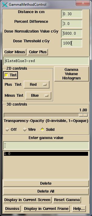
Gamma method control tool.

Using this tool you can display iso-gamma curves on 2D images or an iso-surface in 3D perspective views. The image must contain an image from the stacked image set or one fused to it. You must type in the reference dose in cGy. This reference dose is also used elsewhere in the program to compute dose difference percentage for specifically selected points. Initially the program will default to the largest planning system dose (before 23 June 2016, the dose at the average location of isocenter was defaulted to).

The percent of points with a gamma value <= 1.0 will be computed and shown.

Gamma default criteria

The default values for distance and percent may be set in the file GammaDefaultValue.txt in the program resources directory. A example file is shown below (see Gamma Volume Histogram below for a version 2 file format):

/* file format version */ 1

// gamma distance in cm

0.5

// gamma percent

5.0

Threshold Dose

A dose threshold value may be entered that will report the percentage of points <= the gamma value of 1.0 for the dose that is equal or greater than the threshold dose, in a plane. This function is similar to the gamma histogram described below. Here a different threshold dose may be specified for a plane or the histogram. On the auto report, the same threshold dose is used for both.

Hit the “Display in Current Frame” button to display the gamma distribution in the currently selected frame. The currently selected value is tinted (2D) or is the display value (3D). The hot spot is shown on both 2D and 3D displays. Or hit the “Display in Current Screen” button to display the currently selected values on all frames on a screen.

Gamma Reset Button

The “Reset Gamma” button is to force a complete re-computation of gamma.

Example 2D Display of gamma

An example 2D display is shown below:

Note that you can select the colors to show the plus and minus gamma values. The colors selected will be the default in future runs of the program.

Gamma 3D Display

The gamma isosurface may be displayed in a three dimensional view:

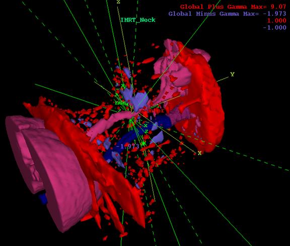
Gamma Volume Histogram

A volume histogram of the gamma function can be computed and displayed.

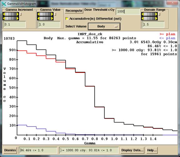
Gamma volume histogram.

An accumulative distribution or differential distribution may be shown depending upon the choice of a toggle button. The distribution may be shown for any selected outline region of interest. Shown here is an example for the entire patient model volume. Bins are created over the range of gamma value at regularly spaced intervals, here 0.1 in the example, and the points in the gamma distribution lattice is sorted into the appropriate bin. Black above shows the total gamma distribution, red the areas where computed dose was >= plan dose, cyan <= plan dose.

For the differential histogram, the volume at the top of the vertical axis will be the volume with the largest increment. For the accumulative, the volume value shown is computed from that covered by the dose matrix and is not necessarily the volume of the region of interest.

The percent of points less than or equal to a selected gamma value (absolute value) is computed and shown. And the same is shown for the subset of points that is greater than (or equal) to a specified threshold dose, in the example above 1000 cGy is the threshold value. These values are shown both in the bottom text fields and on the graph.

The Domain Range control can be used to shorten the range plotted on screen. The “Display Data” will write the data to an ASCII file and display the contents of the file.

As with any frame, clicking the left mouse on the window of the graph (to put focus on the window so that it can receive a keyboard event), and then hitting the P key on the keyboard will allow you to print the graph.

Pass-fail criteria

After June 23 of 2016, a passing criteria can be specified in file format version 2 for file GammaDefaultValue.txt (version 1 shown above).

/* file format version */ 2

// gamma distance in cm

0.5

// gamma percent

5.0

// default passing criteria for percent of volume, in percent

Pass-fail log file

A log can be written out showing pass or fail using the above percent criteria for each volume selected for the gamma volume histogram as described below. For this to occur the folder in which the log file is to be written to must be defined by the file PatientGammaAutoReportLog.loc in the program resources directory. An example file is shown below:

/* file format version */ 1

// path to the folder where the patient report log file is to go

<*g:/PatientLogReport.d*>

/* Set to 1 if the external contour always to be reported */ 1

// otherwise zero and only picked volumes will be reported.

The folder must exist. Simply delete this file to turn off this feature.

Gamma summary web page.

The log file PatientGammaLog.htm will be created in this folder and appended to every time an auto report is generated. The log file is to be viewed in a web browser. A link is provided to the Auto Report. An example entry is shown below:

Doe_John_1234 Plan: IMRT_Neck Date: 08-Mar-2018-21:24:53(hr:min:sec)
3.00% of 5992.0cGy at 0.30cm, 90.00%
pass 66Gy 97.84% <= 1.0 for 2080 pts
pass 66Gy >= 1198.40 cGy: 97.84% <= 1.0 for 2080 pts
fail Body 86.08% <= 1.0 for 103319 pts
pass Body >= 1198.40 cGy: 90.27% <= 1.0 for 39552 pts
pass esophagus 91.36% <= 1.0 for 81 pts
pass esophagus >= 1198.40 cGy: 91.36% <= 1.0 for 81 pts
Auto Report

If this file gets too long, the user can delete it and a new one will automatically be created.

The passing percent value used is entirely the responsibility of the user. And it must be noted that differences between the plan and the reconstructed dose does not necessarily mean a plan delivery is bad. The reconstructed dose should be evaluated in terms of whether the plan is still acceptable. The reconstructed dose might even be an improvement. Be sure to review dose volume dose specifications under Dose Volume Histograms as an alternate method of evaluating a plan.

Difference Dose Volume Histogram

This tool computes a differential volume histogram of the dose difference for a selected region of interest volume. The absolute difference is shown with a black curve. The positive difference, the computed dose greater than the downloaded dose, is shown with a red curve, and the minus difference is shown in cyan. You can toggle off and on each of the three curves separately.

Dose Difference Volume Histogram

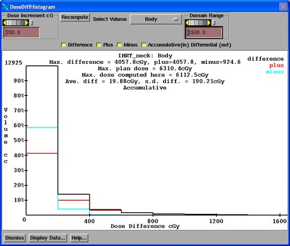
The dose increment control controls the width in terms of dose of each volume element that is counted. The dose is shown along the horizontal axis and the volume along the vertical. Note that the volume is in cubic centimeters and that the dose is in centiGray.

The maximum difference is reported, and then broken down into the largest positive difference and the largest negative difference. The maximum plan dose downloaded is shown next below, and below that the largest dose computed here, for the selected volume.

The recompute button is to be used if the plan is changed without bringing down this popup, and will reinitialize and recompute the curves.

To print, click the mouse in the plot display area and then hit the "P" key on the keyboard.

Show 2D and 3D TPS Dose

There is a option to simply display the dose from the treatment planning system (the reference dose). Select either the Show 2D TPS Dose or the 3D control (see above compare 3D control) under the Evaluate pull down. You then type in the dose value for the isodose curve to be displayed. Then hit the “Display in Current Frame” button. All the isodose curves will be shown in the same color. You can select the color, and also tint the dose for the current isodose value which you can select with the mouse from the list. This also will allow you to show the dose on a fused image set.

Show 2D TPS Dose Control

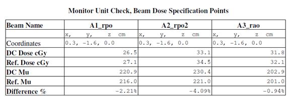
Monitor Unit Check

A monitor unit check can be reported. The monitor unit check is accomplished with the following formula:

DC mu = plan mu X plan dose / DC computed dose

Where plan dose is the planning system reported dose to a point from a single beam,

DC computed dose is the dose that DosimetryCheck computes at the same point,

Plan mu is the monitor units from the planning system for the beam, and

DC mu is the monitor units found from considering the ratio of the dose to the point.

Warning, Dosimetry Check monitor unit is not to be used to treat a patient:

The DC mu is not to be used in treating a patient. This report is only for verification purposes. Any large difference should be investigated and corrected.

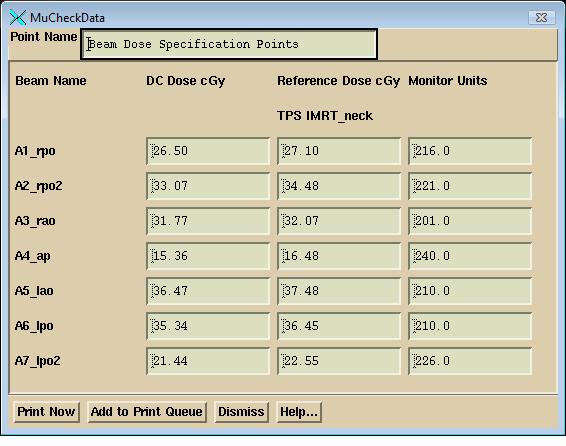
Beam Dose Specification Point

A beam dose specification point is defined by Dicom RT items (300A, 82) and (300A, 84), the location of the point and the dose. If both are present for each beam, then you can base the mu check report on that information. As the beam contribution and monitor unit should be in the Dicom RT plan file which you imported, you should have not to enter any further information. The dose specification point is for one fraction. Each beam will have a separately specified point. The points might or might be at the same physical location.

Specific point

You can alternately select a point from the list of specific points. The beam contribution of the dose to that point from the planning system will not be known from the Dicom RT download, and so you will have to enter those values in the example popup shown below from referring to the planning system. The monitor unit should be known from the Dicom RT download, Dicom tag (300A, 86). If not, then you will have to enter those values as well.

If you leave any field blank, that beam will not be reported on. If you do not enter the mu, then an mu check will not be reported for that beam. Likewise if you do not enter the dose from the planning system for a point for a beam that beam will not be reported on. This mechanism can be used for the case of a different point for different beams. Enter the dose and mu for the beam you want the report for and generate the report. Then repeat this process with the different point and enter the values for the beams to be used with that point and generate a report.

Below is the MUCheckData pop up, shown for the case of selecting to use the dose specification points. After entering any needed data, hit the print button or add to print que button to generate the report.

On the print out you will get the reported percent difference for the dose difference which of course is mathematically equivalent to the difference in monitor units. The monitor unit calculation does not add any new information.

The coordinates are in Dosimetry Check plan coordinates. All doses shown in the version after Feb 4, 2013, will be for one fraction. The dose computed by Dosimetry Check will be multiplied by the # of Fractions/Normalization value shown on the Plan toolbar (see below), and then divided by the number of fractions down loaded from the planning system. The former value is initially defaulted to the number of fractions downloaded form the plan, but then can be changed by the user. The number of factions from the planning system used for division is not changed by any operation. Prior to Feb 4, 2013, the dose was shown for all fractions for specific points.

Show RMU Value and RMU Profile

Two tools are provided on the Evaluate pull down for evaluating the fluence images of the treatment beams. One will simply return the rmu value at any point selected with the mouse. The accompanying Show Pixel Value control is used to get the mouse click location.

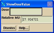
For square open fields, the rmu is equivalent to the in air scatter collimator factor. Hence square fields can be easily used to access the accuracy of converting images to fluence images.

The second tool will show the profile through any flunce image of a beam.

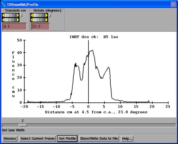
This tool works just like the 1D compare dose tool described above, except here only the profile through a fluence image is shown. Select a fluence image to make it the current frame, and then hit the “Select Current Frame” button. Use the translate and rotate controls to select a line though the fluence image. Then hit the “Get Profile” button. The zero along the horizontal axis is at the perpendicular bisector of the central axis projected onto the line.

Options pull down

On the options pull down are other miscellaneous choices.

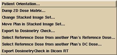
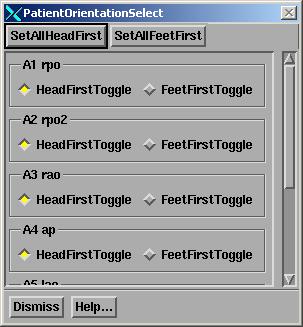
Patient Orientation

The patient may be specified as head first or feet first on the treatment couch. This is a beam attribute but the choice is here so that one can easily set all beams to the same patient orientation. This has nothing to do with how the patient is scanned. This specifies how the patient is placed on the treatment table for a particular beam. The Dicom RT protocol is capable of specifying a feet first patient, but we don’t believe that the RTOG protocol can be or has successfully been implemented to portray a feet first orientation. Supine versus prone is not a choice. The patient must be scanned in either orientation and will be displayed accordingly.

Dump 2D Dose Matrix

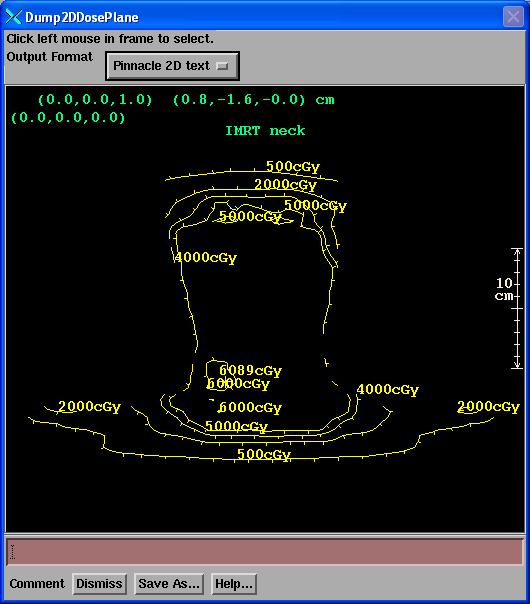
The two dimensional dose matrix for any viewed plane may be written out in an output file. At present the format for that file uses the format Pinnacle (trademark product from Philips, Andover, MA) uses so that other third party software written to read that format can also read the files written here. Select this option from the Options menu.

Click the mouse on the image where the reconstructed dose is shown. Then hit the “Save As” button and navigate to where you want to save the file and also enter in a file name. The output file is a text file. There is currently only one output format choice.

Change Stacked Image Set

Each plan is associated with a primary stacked image set. The primary stacked image set defines the CT number to density conversion and the body outline region of interest (ROI) that defines what is inside and outside of the patient. The primary stacked image set can be fused to other image sets so that the dose computed on the primary stacked image set can be shown on the fused image sets.

However, here is provided an option to change the primary stacked image set. The purpose might be to compute the plan on a cone beam CT data set, for example. In switching the primary stacked image set, the plan and accompanying data structures such as the beam isocenters and dose matrix from the planning system will not likely be in the correct location. You may have to move the plan in the stacked image set as sequentially described below.

We recommend that you first copy the plan so that you keep the original plan coupled with the original stacked image set.

Warning: do not confuse the plan move to a different stacked image set with the original

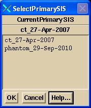
stacked image set the plan was developed for and for which the planning system dose was computed. When you choose this option, the program will present you with the list of stacked images sets under the patient’s entry. You will first have to create and import the stacked image set you wish to use. The selection pop up will show the name of the present primary stacked image set and the list of choices available:

Move Plan in Stacked Image Set

A mechanism is provided to move all the beams simultaneously within a stacked image set, and to also move the 3D dose lattice that was downloaded from the planning system. This might be necessary upon selecting a new primary stacked image set to properly position the beam and 3D dose lattice within the stacked image set.

Warning: do not confuse the moved beams and dose lattice with the original plan.

You might want to consider copying the plan first.

A pop up is provided to accomplish the move:

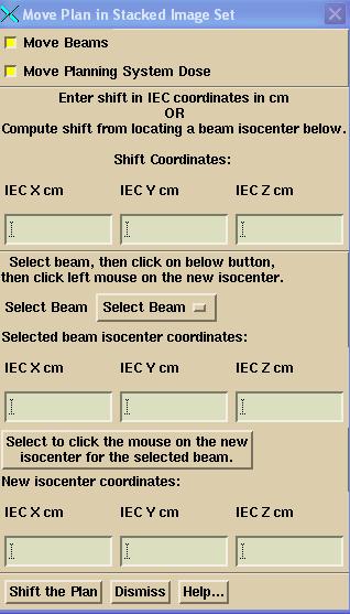
You may select to move only the beams or only the plan 3D dose matrix, or both with the provided toggle buttons.

The shift, if known is to be typed into the Shift Coordinate text boxes, in cm, in the IEC coordinate system: for the supine head first patient, X is your left to right looking into the gantry, Y axis is toward the patient’s head, the Z axis is up. The values shown in the text boxes are the values that are used for the shift. You may select a beam with the Select Beam option menu. The beams coordinates will then be shown in IEC coordinates:

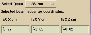
You may then hit the button:

Your cursor will change shape to a plus. If you then click the left mouse on a point in any image of the primary stacked image set, the location will be shown in the “New isocenter coordinates” text boxes and the shift will be computed to move the isocenter of the selected beam to this new point and will be shown in the “Shift Coordinates” text boxes. Only hitting the “Shift the Plan” button will actually move anything.

Export To Dosimetry Check

This is an option that will allow you to export the dose that Dosimetry Check computes to a new plan in Dosimetry Check whereby the Dosimetry Check dose computed in the present plan becomes the imported reference dose in the new Dosimetry Check plan. This feature is provided for the situation where one might want to compare the dose Dosimetry Check computes to some change, such as different input rmu files, different size dose matrix, or what ever other reason there might be. The user has to assign a new unique name to the new Dosimetry Check plan that is created.

Warning: do not confuse the reference dose in the new plan with dose from the treatment planning system.

The label for the reference dose from Dosimetry Check will start with the letters DC, include the plan name copied from, and the date measured of the fluence files. There is a new label on the points report identifying that the plan dose is a prior Dosimetry Check dose.

Select Reference Dose From another Plan’s Reference Dose

You can select the reference dose from another plan to become the reference dose for the current plan. There is no checking if doing so makes any sense or if the reference dose is for the same stacked image set. You are entirely in control of what you want to see.

Select Reference Dose from another Plan’s DC Dose

This option will select to be the reference dose the computed dose from another plan. This is equivalent to the Export to Dosimetry Check function above except that a new plan is not created here.

Export DosimetryCheck in Dicom RT

This option will provide a means to export the dose computed by DosimetryCheck to a Dicom RT file. In addition, all the Dicom files imported can be selected to be re-exported as well. On the export pop up shown below:

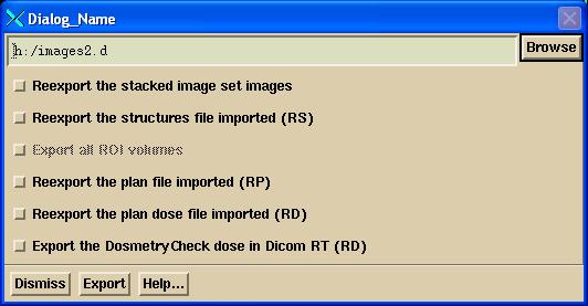
Hit the Browse button to navigate to a directory where the files are to be written to (you can create a new directory), or type in the path (all components must exist). Select the files to export and then hit the Export button. The doses will be multiplied by the number currently in the number of fractions/normalization text box on the plan toolbar. If equal to one dose summation type will be FRACTION, otherwise PLAN.

Hardcopy

You can print a report using the screen capture method and adding comments. See Printing on the System2100 manual. You can keep a running document by selecting to “Add to Print Que”. This will keep a running page count for your document.

Auto Report

There is also an Auto Report facility. The Auto Report will add to an existing report that you may have started. Select Auto Report from the Hardcopy cascade under the Evaluate pull down. This facility provides a method to specify the report up front and leave any calculation time to the computer to perform when the Print button is hit at the bottom of the control. The top half of the scrolled area of the control is shown here:

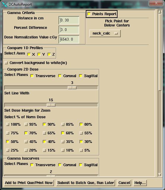
Simply select the features you want written to the report. However, you must select a point. The image planes drawn and profile lines will contain this point. It will typically be isocenter or a dose prescription point. You must also enter criteria for the gamma method. Values entered here are passed on to the gamma method control and vice versus. Be sure that you have entered the number of fractions before using this tool.

The X, Y, Z axes for the 1D Profiles refers to the IEC coordinate system where the Y axis is toward the patient’s head, Z axis is posterior to anterior.

The “SetDose Margin for Zoom” scale control provides some means to default the amount the subsequent images are zoomed up. The program will figure the zoom for images based on the 1D profiles through the x, y, and z axes (whether or not you select them to be in the report, they are computed here). The 50% point of the maximum dose along each line is found and set as a limit of the area to show. To this a margin is added that is selected here with the control. If the margin takes you beyond the patient skin boundary, then the patient skin boundary is kept as the limit. The default is a large margin which will zoom the images up to the edge of the patient. If you set a zero dose margin, you will see the image zoomed up to 1/2 the dose area. Remember that these limits are computed from the x,z axis for transverse, x,y for coronal, and y,z for the sagittal view through the point that you selected. If this does not product the area you want to see, then simply use the middle mouse and right mouse on the images to generate what you want to see, and use the image print facility to make your own report (click left mouse on an image, then hit the P key on the keyboard). Use the separate controls under the Evaluate pulldown.

In the Compare 2D Dose control, the program will also plot any isodose levels that were entered on that control in addition to any values selected here as a percent of the dose normalization value. The largest value that is actually plotted will be tinted.

Below is the bottom half of the Auto Report control:

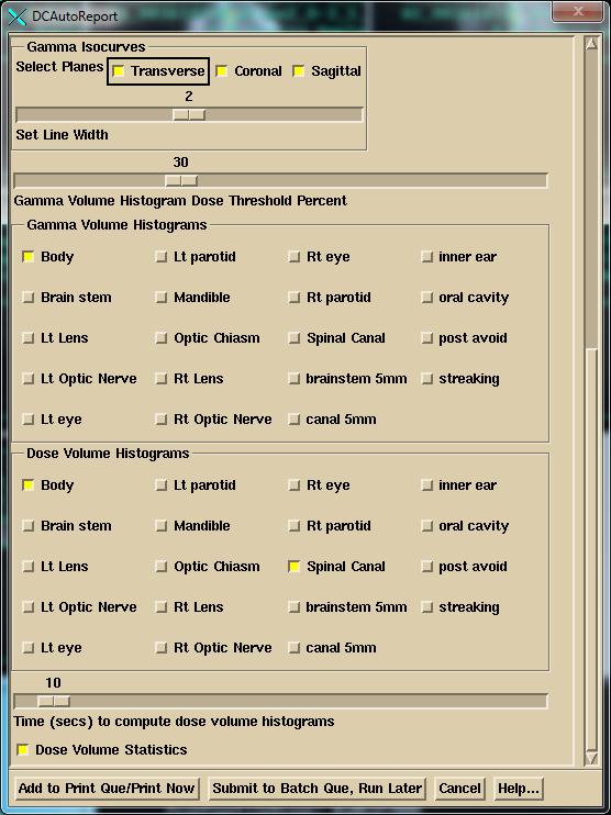
Likewise the 2D gamma isocurves will include any values entered on that control but will always plot and tint the value of 1.0. The Dose Threshold Percent will give statistics for all doses greater than that percent of the normalization dose entered at the top of the pop up on the plane display of gamma and the gamma histogram.

Lastly note the time scale for Dose Volume Histograms. This is the running time for which points are generated to plot the curves. In successive runs for the same selected volumes, more points will be added.

You choices will be remember the next time you run the program.

Default ROI Volumes Selected

In addition, you can specify names of ROI volume to be selected by default the first time you select Auto Report for a plan. In the data directory (specified by file DataDir.loc in the program resources directory, in turn specified by the file rlresources.dir.loc in the current directory) you can create the file AutoReportDefaultNames.txt with the format:

/* file format version */ 1

GAMMA

external

Body

esophagus

cord

DOSE

external

Body

<*brain stem*>

<*Spinal Canal*>

The file follows the ASCII file standard for this program (see the System2100 Manual under the Program Resource Files section). After the format version you may list the names of ROI volumes. Use the keyword GAMMA to specify names for the gamma volume histogram and DOSE for the names for the dose volume histogram. Those two keywords can be in any order and repeated if need be. The names are case sensitive and spaces matter. If a name has a space in it, use <* to *> to set off that name as a single name. Only exact matches will be selected. You of course may make further selections on the Auto Report pop up. This feature is available if ROI volumes are given consistent names across patients.

Submit Auto Report to the Batch Que

On the Auto Report popup at the bottom, you can choose either to compute the dose and generate the auto report now, or submit the task to the batch que to run later. Because it is not a good idea for two or more processes to be writing to the same patient directory, Dosimetry Check will exit at that time. You may then add other tasks to the batch que.

But the BATCH QUE is NOT started when you submit a job. You must hit the "Start the Batch Que Program" button on DosimetryCheckTasks to start the que running. When the last job is finished, the batch que will stop running and will not run again until you start it again. To see if it is running, use the Windows Task Manager and look for BatchQueProgram or the linux ps -e command. Hitting the start batch que program button again will have no affect if it is already running as a lock file prevents a second instance.

# Fractions/Normalization

Use the text field to type in any positive non-zero number that you want to multiple all the doses computed by Dosimetry Check. You can use this if, for example, the 3D dose matrix from the planning system was for more than one fraction. In that case you would enter the number of fractions here. Or there may be some reason why you want to change the computed dose. You could use this factor to force agreement at some point and then consider the agreement of the now relative dose distributions. The default value is 1.0.