Introduction
The Field Dose (Fluence) Toolbar is accessible from any of the Convert****Images programs if there is a need to perform some function. However, images are added automatically in Dosimetry Check for all images saved for the same beam, and adding need not be performed here. Most of the functions below are for entry from the use of x-ray film or a similar process. However, functions are available under the Fluence Functions pull down to process images from electronic devices processed by a Convert****Images program.
It should be understood that in general we are referring to images that will define the fluence map of a field, or otherwise defined as the source model. How ever, these functions could be used under some circumstances for processing dose although there are no analysis tools provided. Hence in this document the term dose and fluence are used loosely.
This program will read in an image of an integrated radiation field and provides tools for converting the pixel values of the image to a dose unit of the user’s choice using a calibration curve. The result is written to a file under the patient’s directory which may then be used by other applications. Tools are provided:
· for locating the field center, orientation, and distance (magnification).
· for creating a calibration curve.
· for calibrating a step strip, and using a step strip to generate a calibration curve.
· for using the calibration curve to convert pixel values to dose.
· for rescaling a calibration curve to force agreement with a single point.
· for piecing together a single field image from multiple images of parts of the field.
These functions may be provided as a separate program called FieldDose, or as part of another application. In either application, selection of Field Fluence will lead to the Field Dose (fluence) toolbar.
Field Dose (Fluence) Toolbar
|
Field Dose Toolbar, showing a field image and BEV’s locator axes partially located. |
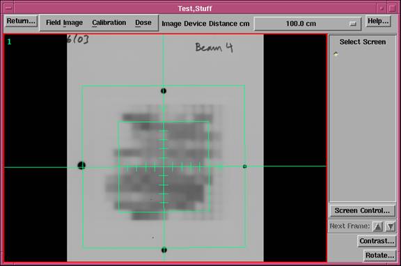
A patient must be selected before the Field Dose toolbar can be used. A bogus patient can be created if doing work that does not involve a patient. Shown above is the Field Dose toolbar. Under the Field Image pull down are options to read in a field image, locate the field, and show pixel and dose values. Under the Calibration pull down are options to create calibration curves and step strips. Under the Dose pull down are options to convert to dose and save the result, as well as functions to piece together a field from multiple images. There is also an option to normalize the field to a point measurement and to display isodose curves.
Read Field Image
To read in a field image you must first select a frame to
put the image into. Simply click the
button that is holding an empty frame.
If there is no empty frame, hit the Screen Control button on the lower
right hand corner and make a screen.
Then select one of the frames.
Under the Field Image toolbar select the type of image. At present the image must be in Dicom,
Tiff, PNG format, or a proprietary
format from Radiological Imaging Technology (
Tiff and PNG formats do not necessarily specify the pixel size but the pixel size is usually include in the file. If not, you must either know the pixel size or it can be determined when you locate the field. However, you must then know the distance that the image was taken at to determine the pixel size and the dimension of something in the image. A Dicom file should include the pixel size in its data. Program rlDicomDump provided can be used to display the contents of Dicom files if you are familiar with the Dicom standard.
We do read 16 bit TIFF gray scale images, which is what most film scanners write.
We have noted that some software (IrfanView) with film scanners will pack a 12 bit gray scale into at 24 bit true color pixel (2 most significant to red, 5 to green, 5 to blue). We have implemented one scheme to unpack a tiff image with 12 bits encoded in the red, green, and blue fields. Since this kind of packing is not part of the Tiff standard, it will work only for this specific case with a 12 bit scanner.
The PNG file format does go up to 16 bit gray scale and we have implemented a PNG gray scale file reader.
From the file selection popup, select the file to be read. If there are no errors the image will appear in the frame you selected.
Locate Field
|
Locate Field Popup |
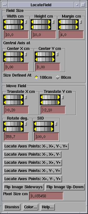
You must first select a frame that holds an image on which you must locate the field. You cannot convert a field image to dose unless the field has been located. The locate field popup will draw the field on the image. The locate field popup has controls to specify the field width and height. For asymmetric fields you use the central axis at control to move the central axis within the field. You should know the field size and asymmetric jaw settings of the field and set the corresponding values. Field sizes are typically defined at 100 cm, but if at 80 you have the option to select 80 cm with the toggle button. We generally always refer to a field size at the distance of definition, i.e. 100 cm, rather than the size at the distance where the field enters the patient.
The bottom half of the control is for the purpose of moving the field within the image. If you know the distance to the image, set that first with the SID (Source Image Distance) control. Then translate the image and possibly rotate it until the field edges line up with the edges of the image. Note the pixel size at the bottom of the control. It defaults to 0.1 cm if the pixel size were not in the image file, and you will be warned in a popup that you must specify the pixel size.
You can default the SID to something other than 100 cm through the use of a file and an option menu on the FieldDose toolbar. This is a convenience for the case of taking images routinely at a distance other than 100 cm. Write a file with the name ImageHolders and put the file in the program resources directory (pointed to by file rlresources.dir.loc). The file format is as follows:
/* file format version */
1
// description, followed
by distance in cm
<*Film holder 1*>
64.5
<*Film holder 2*>
59.8
<*couch top*> 100.0
You can have as many entries as you desire. In the example above, you might have two accelerators for which the source to image distance is different for a film holder that attaches to the collimator. On the toolbar you would then select the film holder distance with the option menu. When the LocateField popup comes up, this will be the default distance showing in the SID field. You can change it from there. This mechanism simply provides a way to not have to type in a distance different from 100 all the time. If the file does not exist the option menu will simply show 100.0 cm as the only choice for a default distance.
If the field is blocked with an irregular field block so that the edges of the field defined by the collimator are not visible, you will need visible marks from which the center and rotation of the field is known. For marks on the axes on the field image, you have the option of clicking the mouse on those points rather than manipulate the wheel controls to align the field locater with the marks. The program expects you to enter points in the order of x-, x+, y-, y+. By x- we mean a point that is negative relative to the point x+ on the BEV x-axis. The same concept for the y axis. If there are only three points, than pick the combination that you have from the buttons shown. The cursor will turn to a left arrow when it is expecting you to hit x-, right arrow for x+, down arrow for y-, and up arrow for y+. The program will fit the BEV axes location to the points entered. You can still continue to move the field afterwards with the coordinate wheel controls.
Match the field size with the field size width and height control. Use the margin control to include as much area around the field as possible up to at least 2 cm. This extra area includes the penumbra and tail area of the beam and must be included if the dose in the area just outside of the field is to be accurate. But exclude any extraneous marks such as fudicial marks, because they will otherwise show up as dose.
A flip image button is available for the case if the image were digitized from the wrong side. The image must be viewed from the source side, that is, as if your eye is at the source of x-rays.
Warning: must properly
locate field in beam’s eye view:
It is imperative that you locate the field in beam’s eye view
coordinates for the Dosimetry Check application.
For the unrotated collimator, the x axis goes left to right across the couch when standing looking into the gantry. The y axis points along the length of the couch toward the gantry. This is known as IEC coordinates. If the collimator is rotated, the image rotates with it. If the imaging device is not physically attacked to the collimator, we suggest that you always make the image in the same setup with the collimator unrotated. Further, you should then have some marker that shows up on the image to confirm the orientation of the beam’s eye view coordinate system. With film in ready pack you might consider pin pricking the x axis with two dots and the y axis with one dot just outside the field. When used with the Dosimetry Check system, if you rotate the coordinate system incorrectly here, it will be rotated incorrectly when applied to the patient image set. This may cause failure to detect a wrong collimator rotation if the field image is otherwise rotated such that it compensates. If the imaging system is attached to the collimator you will have less to do. The center and orientation should be constant relative to all images taken with the device.
As the controls on the Locate Field popup are moved, the field will be drawn accordingly. The color button at the bottom of the popup is for selecting the color that is used after this control is dismissed.
If the source to film distance is unknown, you can change the SID until the beam edges match the image. If the film distance is known but the pixel size is unknown, you can type in different pixel sizes until the beam edges again match up. In general, you should know the pixel size or it should be included in the image file.
You can dismiss the FieldLocator popup when done. Each image in a different frame has its own locator tool. If you simply click the mouse on the next frame when the locator is up, the locator will go down and you will get the locator for the next image. This saves you the step of having to go back to the pulldown menu.
Show Pixel Value
|
Show Pixel Value Popup. |
This tool is used to display and measure the pixel value in images. It is also used with other functions when pixel values are needed from an image, such as when generating a calibration curve using a calibration image such as a calibration film. At the top of the popup is a toggle button for measuring upon mouse release. If selected the area will be measured after dragging with the mouse to the desired location when the mouse is released, making for rapid measurements. Otherwise, one must hit the Measure button to make a measurement. The measurement will be inside the area drawn on the image. The area may be a square, rectangle, circle, or ellipse. The dimensions of the area is controlled with controls provided near the bottom of the popup tool. The dimensions of the area are in the coordinate system of the image at the image distance. When a measurement is made, the average pixel value within the area is displayed, along with the number of pixels that are sampled within the area, and the standard deviation for the average. If this tool is used with another tool, the average pixel value will be automatically transferred to that tool. The other tools that might use this one will pop up this tool at the time the other tools pop up. Used alone, this tool simply reports on the pixel values in images.
|
Show Dose Popup |
Here we have the first example of a control that uses the above Show Pixel popup. This tool is for computing the dose from a pixel value given a calibration curve. Once an image is converted to dose, a different tool is used to simply show the dose from the dose image. The Select Calibration Curve must be hit to select an existing calibration curve. Below we will cover how you make a calibration curve. The pixel value, referred to as the Signal value in the popup, may be typed in or may be found with the Show Pixel Value popup tool. The dose or relative monitor unit is then computed, depending upon the type of calibration curve. The Show Calibration Curve may be used at any time to redisplay the selected calibration curve.
Make Calibration Curve
What we must do here is create a curve that converts the pixel or signal value in an image to a dose value. The calibration curve may be in terms of absorbed dose or relative monitor units. The choice is made with the provided radio box on the popup. The Dosimetry Check program requires that the dose be in terms of “Relative Monitor Units” which we will define immediately below.
Relative Monitor Unit
The relative monitor unit is normalized to the center of the field size for which the scatter collimator factor is unity, i.e. has a value of 1.0. This is typically a 10x10 cm field size as most physicist use this field size as their reference field size. 100 mu applied with a 10x10 open field is 100 relative mu at the center of the field. If the field size is increased to 40x40 and if the scatter collimator factor for a 40x40 is 1.05, then a 100 mu applied exposure results in 105 relative mu at the center of the field. If an attenuator is inserted into the beam, such as a wedge, that attenuates the central ray by a factor of 0.5, then that ray will represent 105 x 0.5 = 52.5 relative mu. The Dosimetry Check program computes the dose from an array of pixel values in terms of relative monitor units. For the above 10x10 cm field size, the relative mu will change off axis due to any change in beam intensity off axis typically caused by the flattening filter.
To generate a curve in terms of relative mu, one can simply set an open field of size 10x10cm, and make selective exposures for different monitor units. The source to image distance (SID) to the image plane must be known and the bolus thickness must remain the same for this and all images taken that are to use the resulting calibration curve. The resulting signal values at the center of the field must then be paired with the monitor units when generating a curve of signal value versus relative mu. The measured signal values must be in a plane perpendicular to the central axis with dmax buildup above the measuring surface. There should not be a phantom below the measuring plane. We want the dose profile to correspond to the in air profile across the field. The build up should not significantly degrade this assumption but in any case it is necessary to record a proper signal free of electronic disequilibrium artifacts. Note that with film variation in film response with depth is not much of an issue as the depth is constant over the area of the film.
Another important consideration is the distance that the relative monitor unit signal values are measured at. We wish to support the possibility of measuring a field at a different distance than the calibration curve was measured at. We must therefore report the distance that the calibration curve was measured at using the text field provided. Suppose the calibration curve was measured at 100 cm and the field at 80 cm. Then the signal values for each pixel of the image will be converted to relative mu from the applied curve and then multiplied by 80/100 squared, since it takes less monitor units to give the same dose at 80 than at 100. The signal value ultimately is the result of an absorbed dose.
Dose
Other uses of this application may require a dose measurement instead. The units of the dose may be specified in the text field provided. A dose measured is the same at any distance and an inverse square law factor is not applied. The Dosimetry Checking program will not accept a field image converted with a dose calibration curve, only relative monitor units can be used.
If the signal value has all ready been converted to dose or relative monitor units as the case may be, a straight calibration curve may be entered, i.e., 0 to 0, 100 to 100, 2048 to 2048, etc.. In any case, the calibration curve must cover the expected range of signal values. The calibration data pairs are fitted to a polynomial curve, and the curve will not be extrapolated beyond the data used to generate the curve. This means that in general, zero must be entered at the bottom of the curve, and the largest signal value anticipated must be included at the top end of the curve.
Signal Versus Dose Popup
|
Signal Versus Dose Popup |
The signal versus dose popup is the tool to use to create a calibration curve. Below calibration curves also may be generated from a calibrated step strip, but initially this tool is used to generate the calibration curve to calibrate the step strip. Curves generated here or from the step strip are the same and may be used equally alike. The signal values may be measured from the image of radiation fields made for this purpose that are read in and displayed using the Show Pixel Value popup. Or signal values may be typed in. The corresponding dose has to be typed in. Then either hit the enter key or the Add To Data List button. The paired data will appear in the below scrolled list area. Individual lines may be selected and deleted. You must select here whether the curve is in terms of dose or relative monitor units. The units of the dose may be entered in the text field. A description of the curve must also be entered by hitting the Description button. When all the data is entered, the Sort button may be used to sort the list in increasing signal value. Then hit the Fit Data button to fit a polynomial curve to the data.
Fit Data
|
Fit Calibration Curve Popup |
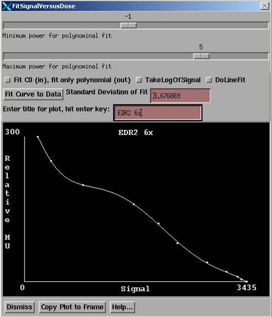
The Fit Signal Versus Dose popup is the tool provided to fit a polynomial curve to the paired signal versus dose or relative monitor unit data. The polynomial may start with negative powers of the signal.
A toggle button controls whether the fitted curve is to approach infinity as the signal value approaches a fitted constant c when fitting a polynomial starting with negative powers. This is to accommodate the case when the dose goes as 1/(c-signal), c > all signal values, when dose increases with increase signal. Or if dose goes as 1/(signal-c), c < all signal values, when dose decreases with increase signal. If the dose increases with signal than x = (c-signal) is used and c is constrained to be larger than all signal values. If the dose decreases with signal, than x = (signal-c) is used and c is constrained to be smaller than all signal values. The software determines the form to use from examining the data that has been entered. Using the constant c in this manner with negative powers of x in the polynomial fit may result in better curve fits to data depending upon the nature of the signal. Otherwise a straight polynomial may be fitted by unselecting the toggle button controlling this aspect and setting the sliders to fit from a power of zero to some positive power.
The range of the polynomial to be fitted is selected by the provided sliders. Let n_min be the minimum power selected with the upper slider and n_max the maximum power selected with the lower slider. Then the polynomial goes from powers of n_min to n_max where n_min < n_max. C is first fitted using a downhill search method if the toggle button is set to fit c. Otherwise c is set to zero and x is set equal to signal. For each value of c during the search, the terms a0 through am below are computed using a least squares fit. The user may change the range of n_min and n_max, except that the number of terms may not be larger than 9 or smaller than 2. The polynomial curve is then fitted:
dose = a0 * xn_m + a1*x(n_min+1) + ... + am*x(n_max)
where the superscript denotes taking x to a power. m = n_max - n_min and n_min < n_max is enforced. Note that n_min may be negative. The default is n_min = -3 and n_max = 3, so with the default we fit a polynomial starting at x to the -3 power to x to the +3 power. a0, a1, ... , am-1, am are the parameters fitted with least squares.
The user may try different ranges of powers for the polynomial fit and try the fit with or without the asymptotic behavior with the constant c to achieve a good curve fit to the data. The curve should run smoothly through the data without any oscillations. Too high a power of a polynomial may cause the curve to have waves in. Generally, if in doubt, pick the lower power. Fit powers 0 to m without c if the curve is not remarkably steep at one end or the other of the domain.
The log of the signal may be taken prior to fitting, although we have not observed any advantage in that. A linear plot point to point may alternately be used, but we believe using a curve fit is better.
A title may be entered for the plot. And the plot may then by copied to an empty frame for continuous viewing. Simply first select the empty frame by pushing the button occupying an empty frame and then hit the Copy To Frame button.
When the data has been satisfactorily fitted to a curve, the popup may be dismissed.
Be aware that the behavior of a polynomial fit outside the range of the fitted data is ill defined. That is, the curve may do funny things beyond the domain of the data used to fit the curve. For this reason a polynomial fit can not and will not be extrapolated.
Warning, calibration curve
must cover signal domain:
Your calibration curve must cover the range of expected signals.
Upon achieving a satisfactory fit, you must save the curve to file in order to be able to use it. Hitting the Save As button will result in a prompt for you to enter a file name to save the curve under. The curve will be saved in a subdirectory CalDCur.d under the data directory specified by file DataDir.loc in the program resources directory. You may create subdirectories under CalDCur.d to organize your data. To delete or reorganize these directories, use the system command language or desk top tools.
Post Signal Versus Dose
|
Post Signal Versus Dose popup |
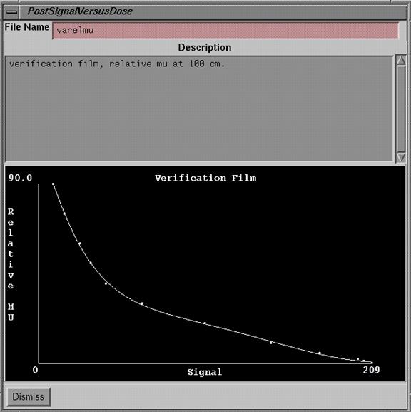
When ever a calibration curve is selected it may be viewed. The popup shows the file name, the description entered for the curve, and a plot of the data and fitted curve. There are no editing tools after a curve is saved. Simply enter a new curve if a change is needed.
Rescale Calibration Curve
When working with film you may correct for processor variations by rescaling the calibration curve. This is accomplished by making a single calibration exposure, typically a 10x10 cm field at the calibration distance to a known dose or monitor unit. Then use an existing calibration curve to measure the dose or relative monitor units to this film. The curve may then be rescaled by multiplying the fit coefficients by the ratio of the true dose (or relative monitor units) divided by what the calibration curve had determined. The origional data used to create the curve is also multiplied by this factor. You simply type in the true dose or relative monitor units in the text field provided
|
Rescale Calibration Curve Popup |
Note that for relative monitor units that the program will not compute relative monitor units until the field has been located, as relative monitor units depends upon the distance measured. But if you know the distance is the same, you can simply type in the result from the dose field.
You must then resave this curve under a new name. Then select this new calibration file for subsequent use. For small changes this method should be sufficient. However, be aware that the gamma (slope) of the response curve can change with film processing. That would require a new calibration curve or use of the step wedge to run a new curve.
Step Strips
When working with film, it may be inconvenient to expose multiple films every time a measurement is to be made. Since film response is known to change with the temperature and chemistry of the film processor, and possibly from one batch of film to another, a calibration is needed when film is used to make measurements. For convenience, we have provided tools to define a calibration step strip, and use the step strip to generate calibration curves for use with measurement films. The step strip might be produced by a step wedge for example. We can use film dosimetry to calibrate the step wedge, and then use the calibrated step wedge in the future to produce calibration curves.
Calibrate a Step Strip
|
Calibrate Step Strip popup |
A step strip is a sequence of constant dose areas as might be produced with a step wedge and a corresponding data structure is created with the calibrate step strip popup. First a calibration curve has to be selected to use to convert the signal values on the image of a step strip to dose. The calibration curve determines if the dependent variable is dose or relative monitor units. If using film, the calibration films and step strip film should be run at the same time.
Normally, one will read in and display an image of the step strip. The show pixel value popup is used to measure the pixel values from each step. Normally start with the beginning step that is to be the first, or number one and then proceed in order to the last step. For each step a signal value must be entered, which can come from the show pixel value popup as mentioned above. The signal value is then converted to dose using the calibration curve. What is saved to define the step strip is the step number and the dose assigned to that step. You can turn off the auto increment in step and enter the steps in any order. From the scrolled list, you can select data pairs to delete. The data pairs can be sorted in increasing order of steps if you did not enter the data in order. Lastly, you must save the step strip under a file name by hitting the Save As button. The step strip will be saved under the subdirectory StSp.d in the data directory specified in the file DataDir.loc in the program resources directory. You may create subdirectories under StSp.d to organize your data.
Use Step Strip
|
Use Step Strip popup |
Once you have created a step strip, you may use it to generate calibration curves. You simply make an image of the step wedge at the same time the measurement image is made. We are not using the word film here because there is no restriction here to film as a means of obtaining images. In any event, since we have a dose assigned to the step strip from above, the dose for each step may now be associated with the signal value from the present step image to produce a calibration curve. The show pixel value popup may again be used to measure each step. By setting the measure on mouse release on, along with auto increment step on, one can measure each step quickly with the mouse by dragging the measurement area to each step and releasing the mouse on each step in successive order. After each step has been measured, the Fit Data button must be hit to fit a curve as described above for any calibration curve. Data pairs from the scrolled list may be selected to be deleted. The Sort button will sort the data in order of increasing step number. A description must be entered for the curve.
To be used, the calibration curve must be saved using the Save As button and then enter a file name. Subdirectories may be created to organize your data. A calibration curve created here is no different from that created above using the make calibration curve popup. The calibration curve generated here may be used to convert the field image to dose or relative monitor units (depending upon the calibration curve used to calibrate the step strip).
Convert To Dose
|
Convert to Dose popup |
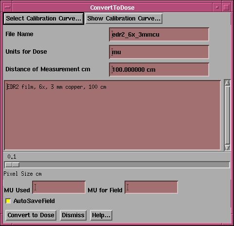
To convert a field image to dose, make the field image the current frame by clicking the mouse on the image. Then click the button in an empty frame where the converted dose image will be shown. You must select a calibration curve from the convert to dose popup. The description of the calibration curve will be shown along with the file name and units for the dose, and distance of measurement.
The dose image will be given a different pixel size starting at 0.1 cm. The slider may be used to select a larger pixel size if there is some reason to do so. At the bottom of the popup are two text fields which provide the opportunity to scale the dose up by the ratio of mu for the field divided by the mu used to make the image. This may be used for the case when the imaging device did not have the dynamic range to record the entire exposure. Hitting the Convert To Dose button will read the selected input image, convert each pixel to dose, and display the resulting image in the empty selected frame. The dose is stored in a floating point array which is converted to an image for display. You must save the converted dose image to a file to use it with the Dosimetry Check function, which save can be accomplished under the Dose pulldown menu. However, leaving the AutoSaveField button in will cause the converted dose field to be saved using the field label as the file name. After the field is converted, a popup will request the field label. You will not have to save the field in a separate operation. If a file all ready exist with that name, you will be prompted to either overwrite the field or cancel writing a file out, in which case you can enter a different label. When you return from the FieldDose toolbar, you will be warned if there are any field dose arrays that you have not saved to a file.
Simply continue to select new frames to convert and empty frames to put the converted image into with this tool up, working through all the located field images. You might want to arrange all the field images on one row, and the converted dose field images in the row below. Later, for DosimetryCheck, on the beam toolbar when you select the dose field file to associate with a particular beam, you might to use a third row to redisplay those images as they are selected. The beam toolbar forces you to redisplay the image file that you are selecting.
Normalize Field
|
Normalize Field popup |
The normalize field popup enables you to normalize a dose image to that measured at some point within the image. You may use a diode or an ion chamber to measure the value. You may use a calibration file to convert a reading to the dose or relative monitor units, or you may type in the value directly. For an ion chamber, you may have the program apply the temperature and pressure correction.
To use a calibration file, hit the Select button to select the file. For an ion chamber, you must type in the temperature and pressure if that option had been selected when the calibration file was created. Type in the reading and hit the Compute Dose or Relative MU button to convert the reading to the dose or relative monitor units.
Once you have the value to normalize to, hit the Apply button, the cursor will change shape. Then click the mouse on the correct spot on the field dose image. Use the Show Dose popup tool to verify that the dose was renormalized as expected.
Make a Dosimeter Calibration File
The tool to make a dosimetry calibration file is gotten from the Normalize Field popup that comes up when selecting the Normalize to Value button on the Dose pulldown menu. The make dosimetry calibration file tool is for the purpose of creating a file that can convert dosimetry reading to dose or relative monitor units.
|
Dosimeter Calibration popup |
Select with the toggle button to select whether or not
temperature and pressure is to be corrected for. A diode would not require correction where as
an ion chamber does. If correcting for
temperature and pressure, enter the temperature and pressure for which the
reading was made.
Lastly, hit the Save As button to save to a file. You will be prompted for a file name. The file will be saved under the directory CalFieldDose.d under the data directory specified by the file DataDir.loc in the program reference directory. You may also specify a subdirectory to organize your data.
Piecing Together a Dose Image from Partial Images
If the image of a field did not fit on one film (or imaging area), you can combine images of different parts of the image to form the complete image. You can also use these tools to simply add the doses from two or more images, or to average the dose from two or more images. These operations are only applied to the image of a dose field after conversion to dose or relative monitor units.
To piece together a single image from partial images, use the below Restrict Area tool to define the valid areas of each partial image. Then use the Combine Dose Fields to create the final image.
Restrict Area
|
Restrict Area popup |
Use the restrict area popup to define a rectangle on a dose image that contains image data. You may do this to reduce an unnecessary large margin to reduce the computation time of a beam. Given the area of the measured field fluence, pencil beams are generated. If the area is smaller, less pencil beams are generated. For example, if you used an EPID image that is 30 x 40 cm in size, pencil beams would be generated over the 30x40 cm area (unless the pencil would miss the patient altogether). If the radiation area is actually some small area, there is no point in computing pencils that have essentially a zero or near zero intensity assigned. Reducing the number of pencils that are generated will reduce the computation time.
Or you may also do this for the purpose of piecing together a larger field from images of parts of a field (on the field dose tool bar). Make a frame with a field dose image current before selecting this option by clicking the mouse on that frame (a red border around a frame is the current frame).
If simply restricting the area, the result is automatically saved to a file if the fluence was read from a saved file. Otherwise you must select to save to a file from the field dose tool bar.
Piecing Together a Fluence Map
If you need to piece together a fluence map, you can only do this from the field dose tool bar. Do this from one of the Convert***Images programs if you used them to process images. In the latter case of piecing together a new fluence field, do not allow the rectangle to enclose an area inside the field for which there is no image data but where data is going to come from another image. Only the areas enclosed in the rectangles from all the selected images will be averaged or added together. Select the dose image by making its frame current by clicking the mouse inside that frame. Use the width and height controls on the Restrict Field popup to control the size of the rectangle. Use the translate controls to move the rectangle about the image. You may alternately use the mouse to drag an area. Just do a left mouse press at one corner and drag to an opposing corner, than release the mouse.
When done, hit the Accept button. The rectangle will be redrawn in a different color from the active color. If you want to change the area, you can always bring the Restrict Field popup back up to change the area, or hit the Delete button to remove the restriction. You can also change the color that the restricted area will be drawn with when the popup goes down. Use the Combine Dose Fields popup to collect the rectangles from different images.
Adding or Averaging Field Dose Images
You can use the Combine Field Dose tool to add or average more than one field dose image to make a new one.
Combine Field Dose
Choose this option under the Dose pulldown menu. Here you can select different frames to add or average together. However, all frames must hold an image of the same pixel size and field size, and be of the same type, dose or relative monitor units.
|
Combine Dose Fields popup |
Using the combine dose fields popup you will build the picture on the popup one frame at a time. First select whether you are adding or averaging the pictures. If you are piecing a picture from sub-pictures, you would normally select average. If you need to add a series of fields to make a sum, select add. For each frame, hit the select frame button and then click the mouse inside a frame. The cursor will change. One mouse click may be needed to make the frame current and the next to select the data in the frame. The entire image will be moved to the popup unless the area has been restricted with the above Restrict Area popup. In that case only the data within the restricted area will be copied to the popup image area. Hit the Cancel Select if you change your mind about moving data from another frame.
The Reset button at the bottom of the popup will allow you to erase the current image and start over again. Once done, you may copy the image to an empty frame with the Move To Frame button. You must move to a frame if you are going to save the dose image to a file.
Show Field Dose
|
Show Field Dose |
To display the dose in a field dose image, use the Show Dose Value under the Dose pulldown menu. The popup again uses the Show Pixel Value popup to measure areas in the selected image. The difference between this tool and that under the Field Image pulldown menu is that here the pixel values of the image are in terms of dose, whereas with the former a calibration curve must be selected to convert pixel values to dose. To display the field dose array as an image, the pixel values must be scaled. However, this does not effect the actual dose stored for each pixel. This popup tool will show either dose or relative monitor units depending upon the source.
Field Label
Select a frame that holds a field dose array. Then select Label under the Dose pulldown menu. The present label for that frame will be displayed if there is one. You may type in a new label. The label will appear at the top of the frame. Use this as a way to clearly label each field image that you have.
Save Field Dose to File
You will not be able to make use of the field dose array produced here unless it is saved to a file. The field dose array will be saved to a file using the entered label when the image data was converted to dose if the AutoSaveField toggle button was in. To otherwise save the dose array to a file, select the frame that holds the field dose array (an image that has been converted to dose) by making that frame current. Then select Save under the Dose pull down menu. You will be prompt to enter a file name. The field dose will be saved under the patient’s directory in a subdirectory called FluenceFiles.d. You may also create subdirectories to organize your data. When this file is selected with the Dosimetry Check program, a copy of this file will be made and stored under the beam that the field fluence belongs to. Each beam will be stored in a subdirectory under the respective plan and the plan is stored under the patient’s directory.
Retrieve Field Dose
Once a field dose has been saved to file, it may be recalled and redisplayed. Select an empty frame to show the image in and then select Retrieve Dose Field under the Dose pull down menu. You will be prompted to select the file name of the field dose. The field dose array may then be renormalized and resaved, for example.
Show Isodose Curves
By selecting Isodose Curves On under the Dose pulldown menu, isodose curves will be plotted through the data. The maximum dose in the array is found and then values are drawn in increments of ten percent. The increments and colors used are in the file TenPercentIsodose in the program resources file. The purpose here is to just show the level of doses that exist and so we have not provided tools to select individual values to show. The label for each curve is the dose value for that curve. To turn off the isodose display select Isodose Curves Off. Only the current frame will be effected by either choice.
Hard Copy
The System 2100 print screen function is used to make a hard copy of any image. Click the mouse in a frame and then hit the Print Screen key on the keyboard. You may print to fit to paper, or select a magnification factor. You can use the mouse on the popup to select an area within the image to print.
Files
If supplied as a separate program, the file name to invoke is FieldDose. A separate license will be needed. The program resource file is FieldDoseRes. This file must be in the user’s home directory or copied to the directory /usr/lib/X11/app-defaults on Linux systems.
Data is stored under subdirectories in the directory specified in the file DataDir.loc in the program resources file. The subdirectories are:
1. CalDCur.d where calibration curves are stored.
2. StSp.d where step strip files are stored.
3. CalFieldDose.d where calibration files are stored for measuring point doses.
The actual field dose is stored under the patient’s directory under the subdirectory FieldDose.d. The Dosimetry Check program will copy each file selected for a beam to that beam’s directory. This will result in at least two copies of the same data, one in the FieldDose.d directory and the second under the particular beam’s directory.
File TenPercentIsodose is read to define the isodose levels to plot when showing isodose curves.
Other required program files are covered in the System 2100 documentation. Deleting old files or directories is performed by the user using the operating system tools on the computer.