This document describes the routine for fitting the pre-treatment deconvolution kernel. There is also a new routine for fitting the exit transit dose deconvolution kernel. The exit dose kernel includes the kernel needed for pre-treatment images, i.e. 0 thickness. Therefore you can use the exit fit routine for pre-treatment images by fitting only for zero thickness. It depends on whether you want to successively have to use the mouse to select the rmu image file, the corresponding point, and type in the monitor units, for each field size (below), or edit a file instead (exit option). The exit fitting program is described in a separate document.

If the deconvolution kernel does not fit your EPID, then you need to run a new kernel fit. If the kernel does not fit, you won't be able to compute the right dose in water. The only way to tell if it fits is to check field size response for different square field sizes. You might consider looking at a 5x5 cm field size and a 20x20 field size, using a 10x10 for calibration.

The EPID looks like a phantom that is denser than water. Signals will be too large for field sizes > 10x10 and too small for fields < 10x10 compared to water (assuming your calibration field is 10x10, it can be different). In other words, the EPID looks like it has a larger back scatter factor than water does. In either case, the deconvolution kernel is needed to convert signal back to in air fluence (rmu). If you are not getting the right dose due to not getting the correct rmu, you need to fit your own kernel. It all goes back to this equation:

Sc,p = Sp X Sc

(dose in phantom) = (phantom scatter factor) X (in air collimator scatter factor)

Please see, for example, equation 10.2 on page 203 in The Physics of Radiation Therapy by Fraiz Khan, second edition; or page 226 in Radiation Therapy Physics by Hendee and Ibbott, second edition.

Sp, phantom scatter, is usually normalized to a value of 1.0 for a 10x10 field size. For Cobalt 60 one can normalize to 1.0 for a field size of 0x0, in which case it is called the back scatter factor.

Our unit for fluence, rmu, here corresponds to the definition of Sc. Consider putting a build up cap on an ion chamber, and reading the signal on the central axis for successively larger square field sizes, and normalize to that for 10x10. That meets our definition of rmu and Sc. However, the buildup cap will distort your values some what. Hence, one instead should compute Sc by calculating phantom scatter Sp, which can now be done with Monte Carlo calculated dose kernels, and divide that into the measured output factor Sc,p to get Sc:

Sc = Sc,p/Sp

Program GenerateBeamParameters in fact does this and writes the Sc table to the file CollimatorScatter06 (here for 6 MV) in the beam data directory for the energy of a particular machine. Because fluence cannot be directly accurately measured, here we work through it and always compare the use of the fluence to a dose in water result.

Since the EPID looks like a phantom (and looks like something denser than water), the deconvolution kernel is needed to convert the EPID signal values back to in air fluence, which is the Sc factor for square field sizes. That is, the Sp factor for the EPID signal is removed, leaving the in air scatter collimator factor (fluence):

EPID signal for square field size = EPID phantom scatter X in air collimator scatter factor

With the correct point spread kernel for the EPID we can calculate EPID phantom scatter and get:

In air collimator scatter factor = EPID signal / EPID phantom scatter.

Then:

In air collimator scatter factor X in water phantom scatter = in water output factor.

where in water phantom scatter is computed with a poly-energetic pencil beam kernel fitted to beam data by program GenerateBeamParameters.

EPID signal / EPID phantom scatter (here on the central axis)

is computed using the inverse of the point spread function for the EPID, which we refer to as a deconvolution, see the JACMP paper where this was developed:

WD Renner, K Norton, "A method for deconvolution of integrated electronic portal images to obtain incident fluence for dose reconstruction", JACMP, Vol. 6, No. 4, Fall 2005, pp. 22-39.

So the only way to know if the kernel is right is to see if you get the correct in air collimator scatter factor for different field sizes which will result in computing the correct dose in water for different square field sizes.

Fitting Deconvolution Kernels for Electronic Portal Imaging Devices (EPID)

To fit a kernel that will be used to convert images to fluence, you will need to correspond a set of integrated images of increasing field size of known monitor units to a known measured dose, or to a set of scanned fields. The field sizes should range from the smallest that can be accurately measured to the largest the imager can handle.

Subsequently to the above cited paper, we have found that it is sufficient to use a single point at depth for each field, as opposed to using a profile scan as was done in the cited publication: Renner, Norton, "A method for deconvolution of integrated electronic portal images to obtain incident fluence for dose reconstruction", JACMP, Vol. 6, No. 4, Fall 2005, pp. 22-39. Using a profile has the further complication that the profile must be precisely centered or the kernel fitting process will try to compensate. The more important effect is the central axis dose, rather then edge response.

The output factors in the present beam data base may be used as a convenience instead of profile scans. The output file has the name OutPut_w00_06 for example, and an example file is shown here and in the beam data section of the Dosimetry Check Manual:

/* file type: 5 = output factors */ 5

/* file format version: */ 1

/* machine directory name */ VarianStd

/* energy */ 6

/* date of file: */ <*07-JUN-2000 15:58:33*>

// cm cm cm cG/mu

// field size SSD Depth output factor

3.00 3.00 98.40 1.60 0.907

4.00 4.00 98.40 1.60 0.92

5.00 5.00 98.40 1.60 0.935

6.00 6.00 98.40 1.60 0.952

8.00 8.00 98.40 1.60 0.977

10.00 10.00 98.40 1.60 1.00

12.00 12.00 98.40 1.60 1.019

15.00 15.00 98.40 1.60 1.037

20.00 20.00 98.40 1.60 1.060

25.00 25.00 98.40 1.60 1.075

30.00 30.00 98.40 1.60 1.086

35.00 35.00 98.40 1.60 1.094

40.00 40.00 98.40 1.60 1.101

Notice that in the above file the points are at a distance of 100 cm, 98.40 cm to the surface. The specification of these points are in cGy/mu and are not necessarily output factors normalized to some field size. It is immaterial what SSD and depth you use for a point on the central axis, but the dose rate must be correct and consistent with the definition of the monitor unit below. To not do so seems to be a common mistake. Not also that Dosimetry Check does not have a source model (since that is what you are measuring) and is normally not otherwise concerned with the dose specification of individual. However, this file is present so that the in air scatter collimator factor Sc can be generated in the dose kernel generation process and used for convenience during appropriate processes, such as a utility that was written for testing purposes that can compute a fluence file for an open field given a field size and monitor unit specification.

The above output file specification must be consistent with the calibration file defining the calibration point in the same data base. Below is the corresponding calibration file Calibration06 for this machine:

/* file type: 4 = calibration */ 4

/* file format version: */ 1

/* machine directory name */ VarianStd

/* energy */ 6

/* date of calibration: */ <*May 2, 2005*>

/* calibration Source Surface Distance cm: */ 98.4

/* calibration field size cm: */ 10.00

/* calibration depth cm: */ 1.60

/* calibration dose rate (cG/mu) : */ 1.000000

You may of course edit beam data to suit your machine. You should run the program GenerateBeamParameters in tools.dir when you have done so. Here you will simply pick the point for each field size integrated by the EPID, using the about output file as a convenience.

Alternately, profile scans can be made of the fields for one or a few selected depths. If the penumbra is significantly different in the x and y directions, than both cross plane and in plane scans should be made. The scan format used here stores the scan data in cGy/mu. Utility programs are provided to convert the ASCII scan files from various water tank scanning systems to this format. Generally, you will have to know the dose rate in cGy for each scan on the central axis and provide that number. The profile scans can be stored in the beam data directory for the particular energy. The file names should indicate the field size and end in “.pro”.

However, in most cases you can fit a kernel using only a single point on the central axis for each field size using the above output factors. Or you may create a profile scan file that consists of a single point for each field size. An example of a file follows below:

// Varian 2100CD 6x

/* file type: 1 = scan */ 1

/* file format version: */ 2

/* machine name: */ <*VarianStd*>

/* energy = */ 6

/* date of data: */ <**>

/* wedge number, 0 = no wedge */ 0

/* field size in cm = */ 8.00 8.00

/* field size defined at isocentric distance of machine= */ 100.000000

/* Source to Surface Distance (SSD) in cm = */ 100.0

// Here z = 0 is at SSD, negative is depth.

/* Number of scans: */ 1

/* number of points this scan: */ 1

/* x, y, z value */

0.0 0.000 -1.600 0.946

Notice that if changing SSD, the dose rate reported must correspond and be consistent.

The use of square open fields is a convenience, as each square open field will represent a sampling of the spatial frequency spectrum. You could choose to some other field as long as you can provide a measured point in cGy/mu some place within the field and integrate it with the imaging device for some known monitor units.

Refer to the ASCII file standard in the System2100 manual. // to end of line and /* to */ are comments which the program ignores when reading the file. Text data of more than one word must be set off with <* to *>. The value must be the dose rate in cGy/mu and must agree with the definition of the machine calibration in the calibration file. This file is to be put in the machine data directory under the proper energy directory. Note that in the above example, the value is for calibration of 98.4 cm to surface where at a depth of 1.6 cm is 1.000 cGy/mu for a 10x10 cm field.

The image file is the image converted to RMU but not deconvoluted with a kernel. When converting the image files, unselect the “Use Deconvolution Kernel” toggle button on the popup for that function.

Other Electronic Devices

It is expected that this same process can be applied to other imaging devices used for integrating beams, such as ion chamber arrays or diode arrays. In the case of such arrays, ideally you would want only enough material to act as an electron shield and not correct for added bolus material.

Select Machine Toolbar

The first toolbar you will encounter will require you to select an accelerator and energy. Shown below is the choose accelerator toolbar.

Hit the continue button after picking the machine and energy.

Fit Kernel Toolbar

The fit kernel toolbar is shown below:

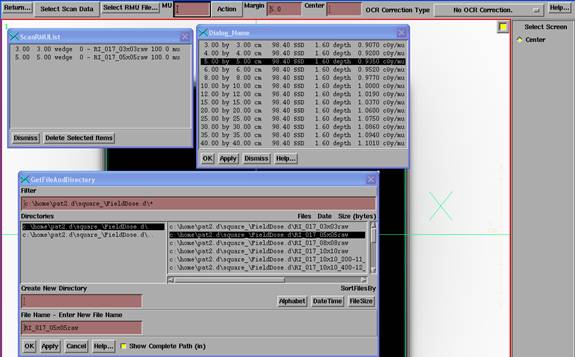
Under Select Scan Data, select either Output Point or Scan File. Here Output Point was selected. Select the point from the output point list read from the above output file and hit the apply button. Then hit the “Select RMU File” button to select an image file. You must then type in the monitor units for the image file in the text box provided on the tool bar. The number you type in is used to multiply the dose rates in the corresponding output point or profile scan file. The entries must be performed in this sequence. A list of point or scan and RMU files with the corresponding monitor units entered will be maintained on a popup. You can subsequently delete individual items from the list, or reset the entire list to zero length with the “Reset List” button on the Action pull down.

Initial Guess File

The default is to fit five exponentials. A default initial guess is provided internally. You can reduce the number of exponentials and otherwise effect the down hill search method by reading in a file with an initial guess for each variable, and control how long the fit process will run. Under the Action pulldown you can select an initial guess file. In the file for each variable must be specified a minimum and maximum range for the variable, the fraction of the initial variable value that is to be the initial step size, and the fraction of the initial variable value that is to be the stopping step size. The step size is halved as the algorithm progresses and stops when the step size for all variables is less than the stop size specified here. It is important that the exponential ranges do not overlay so as to fit separate exponentials.

And example of an initial guess file follows:

/* File format version */ 1

/* file type: 14 = convolution kernel initial guess */ 14

/* Description: */ <*Kernel guess*>

/* machine name: */ <*example*>

/* for energy */ 6

/* number of exponentials */ 5 // two variables per exponential.

// NO ENTRY MAY BE ZERO OR LESS.

/* multiplier exponent */

6.966052e+001 2.288060e+001

8.947527e-002 2.279832e+000

3.360424e-003 6.242489e-001

3.544861e-005 6.401189e-002

4.606968e-008 5.748105e-003

/* min and max value for each variable

Minimum Maximum */

1.0e1 1.0e3 // multiplier

10.0 100.0 // exponent

1.0e-2 1.0e1

0.5 10.0

1.0e-4 1.0e-2

0.05 1.5

1.0e-7 1.0e-4

0.01 1.0

1.0e-16 1.0e-6

0.0001 0.05

/* starting step size fraction, and stopping step size fraction,

fraction of the inital guess above.

step stop */

0.5 .005

An alternate file format version 2 list each variable followed by the minimum and maximum values for that variable, followed by the initial step size and the final step size, repeated for all the variables. The first variable is the multiplier, the second the corresponding exponent, for an exponential, and so on.

Margin

The margin text entry on the tool bar is used to restrict the data used in the fitting process. A positive number will be the distance (cm) beyond the edge of the field for which profile data will be used. A negative number will restrict that distance from the field edge inside the field. There is no reason to make an entry when using a single point on the central axis.

Center

The center text entry provides an additional option to restrict data. Only profile data within the entered distance (cm) from the central axis will be used in the fit. Note above that kernels can be fitted using only a central axis value for the greatest convenience.

OCR Correction Type

There are three options for the Off Center Ratio data. Generally, you would use the third option listed below which is the default. The OCR should be specified out to the largest radius the EPID can measure. The correct option to use must be selected before proceeding and is selected with the option menu on the toolbar, far right. However, the resulting kernel file can be edited later to change this selection. The selection has little effect if only points on the central axis are used in the fitting process.

Multiply in In Air OCR

The first option is to simply multiply the field image after deconvolution by the in air off center ratio. This data will be read from the corresponding file in the beam data directory. This would apply to images which have been corrected by a flood view and have had the OCR removed.

Divide out in water OCR, multiply in in air OCR

A second option is for the case where off axis data has been multiplied in after a flood view correction. The option is to remove that data first before deconvolution. Then afterward multiply in the in air off center ratio as done above. The in water off axis data at dmax is used to divide into the image to remove the same data that was multiplied in. This data comes from the DiagFanLine data file in the beam data directory. We have seen little difference between this option and the third below, which would be to let the OCR data go through the deconvolution process. Further, Varian gives you the option of entering your own data to be multiplied in after the flood view correction. And there is little difference between in water data at dmax and in air OCR data.

Make no OCR correction

A third option is to not make any OCR correction on the image files. The images are simply normalized to 10x10 and then the deconvolution applied. This option would be the case if the OCR has otherwise been multiplied in after the flood view correction or was not removed in the first place. One might calibrate a detector array at a very large distance for instance.

Description

Under the Action pull down, enter a description of the kernel before selecting the fit action. This again can also be edited after the fit.

Fit the Kernel

When ready to run the fit algorithm, hit the “Fit Kernel” button on the Action pull down. As the algorithm runs information will be written out to standard out (the command prompt window if the program was run from the command prompt window) and a popup will maintain the current variable values and the current variance for each iteration.

The length of time can run from one to several hours, depending upon the number of exponentials, the total number of points, and how close the starting value was (and the speed of your computer, we did this on a 1.6 Gigahertz PC), and the size of the image data. Time can be saved by only using profile files that have a profile at dmax only. Reducing the number of points in those files will also save time.

Kernel File

When the algorithm completes, the values of the fitted kernel will be written to a file using the machine name, energy, and the last digit for a file version number, starting with zero. The file will be in the directory DeconvKernels.d in the data directory (data.d) located by the DataDir.loc file in the program resources directory (which is located by file rlresources.dir.loc in the current directory). You might want to rename the file for convenience. The convert programs will remember the file you used prior.

An example file follows:

/* File format version */ 3

/* file type: 104 = convolution kernel */ 104

/* Description: */ <*Fitted Kernel*>

/* machine name: */ <*VarianStd*>

/* for energy */ 6

/* variance for fit = */ 1.246866e+000

/* number of exponentials */ 5

7.040144e+001 2.288060e+001

1.279281e-001 2.762086e+000

8.210560e-004 2.618721e-001

7.239994e-005 5.014250e-002

9.275000e-005 1.477409e-001

/* OCR correction type:

0: divide out in water OCR at dmax, then multiply

in in air OCR after deconvolution

1: multiply in in air OCR after deconvolution

2: make no OCR correction. */ 2

/* file written 09-Aug-2005-13:12:38(hr:min:sec) */

After “number of exponentials” comes the values. The point spread function is modeled with the sum of five exponentials. The first number is the multiplier, and the second is the exponent, for example:

Point spread value = ∑ A e ^{(B x r)}

where A is the multiplier, and B is the exponent, such as:

value = 7.040144e+001 e^{(2.288060e+001
x r)} + 1.279281e-001 e^{(2.762086e+000 x r)} + …

And where r is the radius in centimeters.

Note the OCR correction type that follows. This parameter tells the program whether or not to multiply in an OCR in air correction. This is necessary if the image file does not already contain this correction. The file can be edited and this parameter changed if need be.

Note that in this text file, /* to */ sets off a comment that the reading program will not read. The same applies to // to the end of the line.

Kernel fit results

After the fit parameters come some results (if specific points were used for the fit), all of which is set off as a comment in the file. The first section reads:

/* After Kernel fit.

Field size response of the deconvolution kernel:

Field Size Raw c.a. After Deconvolution Ratio

cm Signal c.a. Signal

4.0 x 4.0 22.69 23.88 1.0524

5.0 x 5.0 22.92 23.81 1.0388

6.0 x 6.0 23.54 24.21 1.0284

8.0 x 8.0 24.40 24.68 1.0115

10.0 x 10.0 24.99 24.96 0.9990

14.0 x 14.0 26.06 25.53 0.9797

18.0 x 18.0 26.69 25.68 0.9621

20.0 x 20.0 27.22 25.95 0.9535

25.0 x 25.0 27.84 25.92 0.9310

The first column above is the field size. Next follows the raw integrated values read from the EPID images. The values are the monitor unit used, normalized by the image file used for calibration, in this case a 10x10 field. So the value for the 10x10 cm field should be the monitor units used for that field.

The raw signal should be strictly increasing with field size.

If not, then you probably have a saturation problem. The integrated value is the sum of multiple frames. Saturation occurs when within a frame the maximum signal value that can be measured has been reached and further radiation within that frame is not recorded. If the same monitor units are used for all field sizes, this is easy to review. In the above example case, 25 mu was used for all field sizes.

The third column is the fluence value after deconvolution in rmu units. Since for open fields the fluence is the in air scatter collimator factor, the values should be this factor times the monitor units. Therefore for the calibration field size, 10x10 cm in this case, the value should be the number of monitor units used. However, it won’t be exact because the kernel is fitted over all the field sizes, each field size representing a sample of the spatial frequency spectrum. There is nothing otherwise special about the calibration field size and we do not want to renormalize the kernel for force exact agreement, unless one ONLY treated their patients with open 10x10 field sizes.

If the value for the calibration field size disagrees by more than a percent from the monitor units (see also the ratio in the last column), there may very well be a systematic error that the fit process is also correcting for. This would occur if incorrect dose rate values in cGy were entered for the points used in the fit. For example, if the calibration method in the calibration file was specified as being SAD (98.5 to surface, depth 1.5 cm, dose rate 1.000 cGy/mu) but the dose rates were entered as if it were SSD (100.0 cm to surface, depth 1.5 cm, dose rate 1.000 cGy/mu), one would see a 3% disagreement here.

The following example clearly has a problem:

10.0 x 10.0 99.97 108.01 1.0805

where we see an 8% error. This was caused by entering points at 5 cm depth that were incorrectly normalized to 1.000 cGy/mu at 5 cm depth for a 10x10 cm field size.

The last column is the ratio after deconvolution to that before. The value for the calibration field size should be close to 1.0. This column represents the field size response of the deconvolution kernel (for the field sizes used).

Next follows the results with the entered points:

In water values.

Field Size Depth Measured Computed

cm cm cGy cGy

4.0 x 4.0 1.50 23.07 23.25 0.77%

5.0 x 5.0 1.50 23.52 23.31 -0.91%

6.0 x 6.0 1.50 23.90 23.81 -0.37%

8.0 x 8.0 1.50 24.52 24.52 -0.02%

10.0 x 10.0 1.50 25.00 24.98 -0.10%

14.0 x 14.0 1.50 25.67 25.78 0.41%

18.0 x 18.0 1.50 26.18 26.11 -0.27%

20.0 x 20.0 1.50 26.37 26.51 0.52%

25.0 x 25.0 1.50 26.77 26.70 -0.28%

The fit is to find the EPID signal after deconvolution, the fluence, here the in air scatter collimator factor, that will produce the correct dose in water for the point specified for each field size that was imaged. Measured is the dose rate what was specified for the point times the monitor units that was entered for each image.

The in water results can be correct but the kernel can be entirely wrong if the kernel has corrected for a systematic error as noted above that occurred from specifying the dose rates to the points used incorrectly.

We would like to see the errors less than 1%. Small fields often show larger errors due to measurement error for measuring small field sizes 3x3 and smaller. The errors represent the accuracy that will be obtainable using the integrating imaging device.

Fit Data File

A file will also be written, “FitDataProfiles”, in the temporary directory, that list the computed and measured values using the initial guess before the fit starts.

Note also that data is written to standard out during the fit. So if the program is run from a command prompt window you will see the progress of the fit and some central axis results at the end of the fit.