Use with the
Varian EPID
6 Sep 2007
Varian
Electronic Portal Imaging Device
Deconvolution
Kernel and EPID Response Variations
Run program ConvertEPIDImages to read in integrated image files from the Varian EPID system and from the Elekta system written by our utility program IviewToDicom.
Run ConvertSiemensImages to read image files from the Siemens EPID system.
Run ConvertPTW2Dimages to read PTW 729 ion chamber images, ConvertMapCheck to read Map Check images, ConvertMatrixxImages to read IBA Matrixx images, ConvertKodakCRImages to read Kodak CR images.
Varian Electronic Portal Imaging Device
Varian’s electronic imaging system supports integration. By integration we mean that the pixel values are summed over the entire beam on time. Hence a 100 monitor unit (mu) exposure will result in twice the pixel values of a 50 mu exposure. The images are to be exported in Dicom format and are read here with program ConvertEPIDImages in that format.
Dosimetry Check will automatically associate the exported Dicom files with the plan beams if the exported files have the beam name in the exported file header for the RT Image Label. Also, it is easier to understand the files if the beam name is in the file name. Set up the Dicom Export Wizard to include the Field ID and Beam Name, by selecting “PATIENT ID + Suffix” when creating the export filter in Varis/Aria.
Wedges
The energy response of the EPID does not give a correct wedge factor for a physical wedge but does give the correct slope. As a work around, a different deconvolution kernel would have to be used for each physical wedge. Hence fields with a physical wedge would have to be converted separately.
Integration Mode
We can provide some information on the Varian integration mode, so that you will know where to look, but you should consult Varian for details
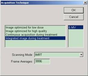
Varis/Aria can handle the details for you. For a manual method in the portal imaging software select “AM Maintenance”. Go to “Maintenance” to “Acquire Image” to “Integrate Image During Treatment”. Select “Start” and turn on the accelerator. The image will pop up on the right side of the screen after beam off. Select “Save All”. The folder where the image is saved will be displayed, such as
c:\Program Files\Varian\Oncology\Treatment\AM\Images\20050601.
File names will look something like SII00286.dcm. You will have to keep track of which file is for which beam.
Another option is to use Varis. Setting this up will enable the beam name from the plan to be assigned to the integrated file names. If a carriage shift is required, you will get the beam name with a number appended in the file name. Dosimetry Check will use the file name to automatically assign the converted files below to the beams in the plan.
Saturation Effect of the EPID
The EPID integrates for a short time period called a frame, and then the frame is read. Integration is accomplished over frames by adding up the frames. If the EPID should saturate during a frame, you will not get correct integration results. This issue was addressed in the publication:
“Performance optimization of the Varian aS500 EPID system”, by Berger, et.al., in JACMP, Vol. 7, No. 1, Winter 2006, pp 105-114.
Of particular interest is figure 5 on page 112 and the NRP parameter. And of particular note are equations (5) and (6) for criteria for setting NRP. NRP is defined as the number of rows read before charges are transferred from pixels to read-out electronics between two accelerator pulses. To avoid saturation, a large NRP must be set. If a shorter SID or higher dose rate is used, a larger NRP must be set to avoid saturation.
The above paper advises that for pulse frequency < 70 Hertz, set NRP = 2.33 X MNR and for pulse frequency > 70 Hertz, set NRP = 4.5 X MNR, where MNR is the maximum number of rows that can be acquired per pulse (see equation 1 in the paper).
One consequence of saturation is that the field size effect is truncated.
Test for Saturation
A way to test for saturation is to integrate for a series of increasing field sizes. The ROI function in AM maintenance is a useful tool for doing this. Shown below are results on an EPID system that is working and one that is saturated.
|
Field Size Cm |
Raw data Not saturated |
Normalized data Not saturated |
Raw data Saturated EPID |
Normalized data Saturated EPID |
|
5x5 |
-5370 |
0.929 |
-7836 |
1.000 |
|
10x10 |
-5781 |
1.000 |
-7835 |
1.000 |
|
25x25 |
-6230 |
1.078 |
-7846 |
1.001 |
In the third column we see the typical field size effect. The dose gets larger with field size for two reasons: an increase due to the in air collimator scatter factor increasing with field size, and an increase due to increase back scatter and other effects in the EPID. The EPID looks like a phantom more dense than water, hence a greater field size effect than would be measured at dmax in a water phantom. In the last column the EPID is clearly saturated. Even for the 5x5 field size, each frame has probably reached a maximum signal value before the frame is read out. So with more radiation per frame with the 10x10 and 25x25 fields, the EPID is not able to measure any more radiation intensity and all fields end up with the same integrated value. One will still see an increase in dose with increase in monitor units because there will be more frames added together for a longer irradiation time. But the integration would not be accurate and useable.
If the EPID settings can be independent of the accelerator dose rate, then another possibility for a test would be to set a large field size and integrate at the normal dose rate used, say for example at 400 cGy/min. Then integrate a second time for the same monitor units but at half the dose rate, say at 200 cGy/min. The integrated value on the central axis should be the same. This test should be at the source image distance normally used. Any change from the test condition that would increase the dose rate at the surface of the EPID could be saturating the EPID.
The below table shows a typical response of the EPID with field size in the second column:
Table 1: Typical EPID results
|
1 |
2 |
3 |
4 |
5 |
6 |
7 |
|
Field size cm |
EPID Raw Integration for 100 mu at 105 cm SID |
EPID values after decon- volution, Sc x 100 |
User Measured Sc with 6x buildup cap, x 100 |
Sc x 100 Computed from Sc = Output/Sp |
Output Dmax water measured for 100 mu |
Output Dmax water computed for 100 mu |
|
2x2 |
86.4 |
88.7 |
92.4 |
|
82.4 |
83.5 |
|
3x3 |
89.3 |
90.9 |
94.1 |
93.8 |
86.7 |
87.5 |
|
5x5 |
93.4 |
94.5 |
96.9 |
95.7 |
93.2 |
92.2 |
|
8x8 |
97.9 |
98.4 |
99.0 |
98.5 |
98.0 |
97.6 |
|
10x10 |
100.0 |
100.2 |
100.0 |
100.0 |
100.0 |
100.1 |
|
15x15 |
103.4 |
102.3 |
101.3 |
102.5 |
103.5 |
103.5 |
|
20x20 |
106.3 |
103.7 |
102.0 |
103.6 |
106.0 |
106.2 |
|
30x30 |
109.9 |
104.4 |
102.8 |
104.3 |
108.8 |
108.8 |
If integration results in nearly the same value for all field sizes, the EPID is probably saturating.
Setting NRP
To set the NRP, one must log into the AM maintenance mode using a service ID and password. The user interface looks like:
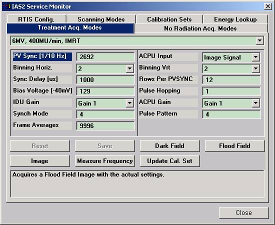
Rows Per PVSYNC is the NRP value. We do not have sufficient information to advise on the optimal settings for these parameters.
Deconvolution Kernel and EPID Response Variations
You will need a deconvolution kernel to convert integrated fields back to in air fluence. You probably should take all your data at the same EPID SID (source image distance). There may be some variation between centers and some small changes with the calibration of the EPID. Therefore you probably should perform your own kernel fit periodically as needed. See the reference manual on fitting a deconvolution kernel. After the deconvolution of square open fields, the RMU values in the center of the fields should reflect the in air collimator scatter factor normalized to 10x10.
Above in Table 1 in column three is the integration values after deconvolution. These values are now equivalent to the in air scatter collimator factor (here x 100). We define the in air scatter collimator factor Sc by the equation:
Output factor = Sp X Sc
Where Sp is the phantom scatter, and the output factor is the dose at depth of dmax. Note that measuring the Sc factor is subject to systematic error due to the need for a buildup cap, which acts like a phantom, and so is not a true in air measurement. Hence the measured Sc factor in column 4 does not agree with that computed in column 5. A pencil beam algorithm is used to compute the phantom scatter Sp, and that is divided into the measure output factor to get the in air collimator scatter factor Sc. Deconvolution of the EPID integration fields is necessary to produce the in air fluence, which is then used as input to the dose algorithm. Hence the in air fluence in column 3 is used to compute the dose in column 7.
Lastly, it has been our experience that measured output for 2x2 fields is generally accompanied by a large uncertaintly if an ion chamber is used, and generally is too small a value.