Quick Start for Dosimetry Check and EPID
Quick
Start for Dosimetry Check and EPID
Calibration
of your Accelerator
Integrate Each Treatment Field
Convert Integrated Field Files
Restrict Area of Fluence File to
Use
Assoicate Beams with the Integrated
Beam Files
Reading
Fluence Files into the Beams Manually (not IMAT)
Leave enough margin around the
fields.
Associate the correct measured beam
fluence file with the correct beam.
Calibration of your Accelerator
You have to review how you calibrate your accelerator as to whether it is 100 cm to the chamber or to the water surface, for your definition of where is 1.0 cGy/mu (or any number that defines your monitor unit at some specified SSD and depth).
Generic beam data is provided and should be sufficient since field flatness is something that comes with the measured fields. Accelerators are in the directory bd.d with one directory entry per machine (start at c:\mathresoluitons Windows or /home/dc on unix). Navigate to a particular energy subfolder and review the file Calibration06 (06 here for energy 6 MV). An example file is shown below:
/* file
type: 4 = calibration */ 4
/* file
format version: */ 1
/*
machine directory name */ Varian
/*
energy */ 6
/* date
of calibration: */ <* 22 April 2005*>
/*
calibration Source Surface Distance cm: */
98.4
/*
calibration field size cm: */ 10.00
/*
calibration depth cm: */ 1.60
/*
calibration dose rate (cG/mu) : */ 1.000
Note that
the above file specifies an SAD calibration.
For an SSD definition the 98.4 entry would be replaced by 100.0.
Either
change the file as described below, or run program DefineMonitorUnit to
accomplish the same operation.
If you need
to change the file do so. On a Windows
machine use something like WordPad to edit a text file. After changing this file you must run program
tools.dir\ComputeCalConstant.exe. The
directory tools.dir is in directory c:\mathresolutions or /home/dc where you
loaded Dosimetry Check.
ComputeCalConstant.exe is an ASCII program which you must run in a
command prompt window.
In Windows
after changing directory to mathresolutions (cd
c:\mathresolutions) just type the command:
tools.dir\ComputeCalConstant.exe
In Linux and
Unix it is:
tools.dir/ComputeCalConstant
You must
repeat this procedure for each energy you are going to use.
Wedges
The energy
response of the EPID’s does not give a correct wedge factor for a physical
wedge, but will give the correct slope.
As a work around, a different deconvolution kernal would have to be used
for each physical wedge, with those physical wedged fields processed
separately.
Integrate
Each Treatment Field
Put your
EPID into integration mode and save each beam integration to a separate file
using a file name that you can associate with each beam in the plan. Varis/Aria will put the beam name from the
plan into the file name if you select the suffix Field ID/Beam Name in the
export wizard. Dosimetry Check can find
the files automatically for a beam if the beam name is in the file name (after
conversion below).
On the
Elekta system, you must select the mode to write segment out as a separate file
during integration. Then run program
IviewToDicom to read in and assemble the segments for each beam into one Dicom
file. Then run program ConvertEPIDImages.
For a
Siemens machine, run ConvertSiemensImages (which uses the same interface
described below).
In
Air OCR
For Varian
we are assuming that the off-axis ratio is being multiplied in by the EPID
software since the flood view removes that.
If not, you should measure the in air off axis ratio and store it in the
proper format in the beam data directory.
You will have to use a different kernel file than that specified below
as the choice of whether or not to multiply in the in air OCR is made in the
kernel file.
Calibration
Field
Shoot an
extra 10x10 cm field for known monitor units.
If you don’t have the exact arm Varian EPID, you will need a separate
10x10 field at each gantry angle since the EPID can shift some as the gantry
rotates. The 10x10 is used both for
defining the central ray and for calibation to monitor units. If you shoot all your beams at 0 gantry angle
or have the exact arm, you need only one 10x10 cm field for calibration and
centering. Use the letters “cal” within
the beam name for calibration files so the letters “cal” appear in the
integration file name. ConvertEPIDImages
will then be able to automatically recognize a calibration file from one to be
converted.
For IMAT,
there is presently no correction for movement of the EPID during gantry
rotation unless you can generate a 10x10 at each gantry angle that is
integrated.
Download
the Treatment Plan
Next run
program ReadDicomCheck or ReadRtogCheck to download the plan in DicomRT or RTOG
format. Refer to the sections in the Dosimetry
Check manual for instructions on how to use those two utilities. The Dicom RT protocol can specify which ROI
is the external body skin contour. The
RTOG protocol has no such method.
Neither specifies CT number to density conversion. ReadDicomCheck will read its starting
location for selecting files from NewDicomRTDirectory.loc file in the program
resources directory.
Convert
Integrated Field Files
The
integrated files must be normalized to monitor units and deconvolved for the
effect of the EPID. A 10x10 is used for
normalization, and a kernel file is used for the deconvolution process. The kernel file VarianStd_6x_noCor is
provided for converting images that have the off axis ratio already restored
which will generally be the case for Varian.
The options in a kernel file are to pass the off-axis-data through, to
multiply in the in air off-axis-ratio data, or to first divide out the in water
dmax curve before deconvolution and multiply in the in air off axis ratio data
afterwards. The easiest thing to do is
provide the off axis data as Varian request it but you should use in air data,
not in water data, and use the kernel example here that passes it all
through. However, there is little
difference between in water data at dmax and in air data.
ConvertEPIDImages
Run program
ConvertEPIDImages. A separate manual
exist for this program on our website.
Select the accelerator and energy, and then select or make a new patient
entry. Hit the Convert Images button on
the Read EPID Toolbar. You will get a
file selection box. Select the image
files you want to convert. You will then
get a popup as appears below:
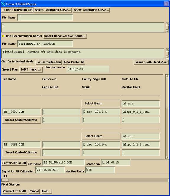
Calibration
The three
methods of calibration are:
1.
To
enter a calibration curve.
2.
To
enter a single10x10 to calibrate and center all fields.
3.
To
enter a separate10x10 to calibrate and center each field.
If method 3
is not present for a beam, then method 2 is used. If method 2 is not present,
then 1 is used if selected, otherwise you get an error message that the program
can’t convert the files. Be careful not
to use an old calibration curve. Delete
an old curve (in data.d\CalDCur.d) or delete the file that stores the name of
the last file used (in data.d\accelerator name\Xenergy.d\EPIDcalFile) if need
be.
When you
select a 10x10 calibration field file, it will be displayed and a method
provided to locate the central ray of the field. Use the name “cal”for your 10x10 calibration
files and ConvertEPIDImages will automatically assign those files as
calibration files and sort them by gantry angle.
Plan and Beam Names
You should
download the plan first for the list of plans available to the patient to be
listed here. Select the Plan. Then for each file to be converted, select
the beam that the file is for. You can
alternately type in these names.
Note the
file names on the right that the converted files are written to. You can change the file names if there is
some reason to do so. The files will be
written to the directory under the patient’s directory ->
FluenceFiles.d
-> plan_name -> beam_name -> IMRT
[or ->
IMAT for arc beams when running program ConvertIMATImages. In that case, you only convert the files for
one beam (arc) at a time.]
If the Dicom
RT label contains the beam name from the plan, this program will try to sort
the files to the proper beam for you, but you must check this for each fluence
file. For the Dicom export (Varian)
wizard, select Field ID/Beam Name as a suffix.
In Dosimetry
Check you will have the option to manually select the fluence files that belong
to a beam. Just select the beam to edit
from the Plan toolbar and look at the Options pull down menu on the Beam
toolbar.
Adding Fluence Files
If you had
to use a carriage shift with your Varian MLC, then you can add the separate
integrated files in Dosimetry Check by simply selecting more than one file for
a beam. Dosimetry Check will add all
files found in the IMRT folder above.
Files in the
IMAT folder are NOT added together.
Rather each is applied at the gantry angle the image was integrated at.
Restrict Area of Fluence File to
Use
Next you may
want to select the Restrict Area function to reduce the EPID area from 40x30 cm
to the size of the radiation field plus a very generous margin to save
computation time later. You can do this
in Dosimetry Check where you will have the option of applying the restriction
on one beam fluence map to all of them.
Run
Dosimetry Check
You have
done the work. The rest is easy. Run Dosimetry Check. Select the patient and then the stacked image
set. Under the Stacked Image Set pull
down select Options and check if the proper external ROI is selected for the
skin contour. Under Density you must
select a CT number to density conversion file.
Select the Marconi curve, but you should eventually make your own. However, dose is not sensitive to this
conversion.
Under
Applications select Dosimetry Check.
Select the Plan. Because this
system is multi-plan, you have to specify where the plan is to be displayed. On the Display pull down you can select a
default screen for a transverse, coronal, and sagittal image through isocenter
or the center of an ROI. You can always
go under the Display pulldown on the Plan toolbar to select to display in the
current frame or screen. You can make
reformatted images on the main tool bar under the Stacked Image Set pull
down. Or you may use any of the images
displayed for the stacked image set.
Assoicate
Beams with the Integrated Beam Files
The program
will attempt to find the files for the beams by looking in the path:
patient_name
-> FluenceFiles.d -> plan_name -> beam_name -> IMRT
If more than one file is found for a beam (in
IMRT), the fields are added. You should
review the images of the beam files that are displayed for correctness. The files used are part of the labeling on
the images that are displayed. Rather,
the label assigned above is the file name by default. You can change the label in the popup shown
above. Each beam will make a copy of the
integrated image dose file. Further
changes in the directory where the integrated fields were deposited will have
no effect. Upon retrieval of a plan, the
program will detect if you have put new files into the FluenceFiles.d path and
give you the opportunity to incorporate the newer fluence files.
For IMAT,
the fields are not added, rather each is applied at the gantry angle measured.
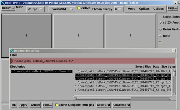
Manually
select fluence files
You can also
manually select the fluence files for a beam and will have to do so if it was
necessary to redo the integration files for some reason. Under the Plans toolbar retrieve the plan
(thereafter select this plan to edit).
On the Plan toolbar select the first beam to edit. Under Options on the beam toolbar, select
“Read Fluence rmu files” if you want the
files added together. For IMAT select
instead “Read IMAT rmu files”. A screen
will be created to hold the images of the beam files or you can create a
screen. Select the file where you stored
the converted field image above and hit the Apply button. You can select more than one file if they
need to be added together (Read Fluence) or for IMAT the files that will
simulate the arc. The program will
display the image, then increment the beam tool bar to the next beam. [Note you can also go directly to any beam's
toolbar using the option menu at the left on the current beam toolbar.] Continue to hit the Apply button being
careful to select the beam file for the current beam shown on the beam
toolbar. On the last beam just hit the
OK button. See below for a picture of
the user interface involved.
Reading
Create
Beams Manually
If you did
not get the beam positions with the RTOG or Dicom RT files, you
will have to
create each beam. The successive beams will
start with the isocenter of the prior beam.
You will have to type in the gantry, collimator, and couch angle under
the Move pulldown on the beam toolbar.
However, because the EPID does not rotate with the collimator, upon
selection of a beam file, the collimator angle will be set to zero.
Be sure the
right energy is selected for each beam.
That should come up correctly with RTOG and Dicom RT.
Pit Falls
Leave
enough margin around the fields.
You need to
leave a generous margin around the fields.
The margin is needed to model the penumbra since the penumbra intensity
comes from the measured field, not a model.
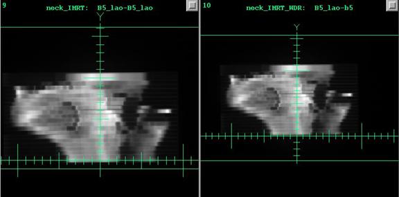
Also, the tail does produce dose within the field as the below images
demonstrate. On the left is a beam (one
of seven) with less margin left then that on the right.
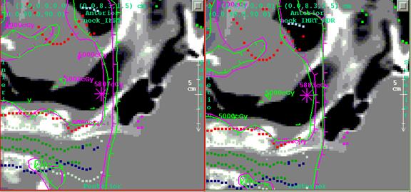
Below on the
left is part of the dose distribution using the beam on the left (one of seven,
all with less margin). On the right is
the plan with more margin. The hot spot
dose went from 5807 cGy on the left to 5883 cGy on the right (for 28
fractions), a 1.3% difference. Notice
the 2000 cGy line on the right (magenta) agrees better with the planning system
isodose line of 2000 cGy (green) .
Associate
the correct measured beam fluence file with the correct beam.
If you
associate the wrong file with a beam, you obviously won’t get the right
dose. In the above images of two
integrated beams, the label shows the plan name, followed by the beam name,
followed by the label names assigned for each image used. These images are displayed as you do the
association for you to check. All images
are shown in beam’s eye view system, x axis to your right, y up. The beam’s eye view system rotates with the
collimator. But the collimator angle
will be reset to zero because the EPID does not rotate with the collimator.
Compare
Isodoses
Return to
the plan toolbar from the beam toolbar.
Under Evaluate select Compare 2D Dose if you got a 3D dose matrix from
the planning system. Make a frame
current where the plan is being displayed on a 2d image. On the top of the compare tool select what
you want to see among dose from Dosimetry Check, foreign dose (from the
planning system), and dose difference. Note
only one thing can be tinted however.
Type in a dose value and hit the enter key. Hit the Display in Current Frame button at
the bottom of the popup.
If you did
not get a 3D dose matrix, then under Evalute select Display Dose in Current
Frame and then select 2D Isodose Lines.
In this case use the same image planes used with the plan and reproduce
the same isodose levels for comparison of hard copy.
Specific
Points
To calculate
the dose to specific points, return to the main toolbar, go under the Stacked
Image Set pulldown to Options, and then select Points. Locate the points with the mouse on images of
the stacked images set. Return to
Evaluate under the plan toolbar and select Point Doses. On the point dose toolbar, select display,
print, or file points. Compare the dose
to the point for what the planning system computed. Note here you can also locate an isocenter
point by specifying the coordinates in beam's eye view, which would be at
(0,0,0).
Gamma
Analysis
Notice the
gamma method under the Evalute pull down.
It operates similar to the Compare 2D doses tool. There is a gamma volume histogram available
also. You have to specify the dose that
the percent is of.
Dose
Volume Histograms
Return to
the Plans Toolbar (one above the Plan Toolbar) and select dose volume
histogram. Select the plan and ROI’s that you want a dose volume histrogram
for. The dose volume histogram computed
from the treatment planning system’s dose matrix will be shown as a dotted
line. The program generates points a
random and computes and displays the curve periodically. Either hit the stop button when the curves
settle down or the program will eventually stop on its own.
Multiple
Fractions
If you
downloaded the dose for multiple fractions, type in the number of fractions in
the text field provided on the Plan Toolbar.
Hard
Copy
To get a
hard copy of any image displayed by the program on the main window or any
popup, click the mouse on the image and then hit the Print Screen button or the
P key on your key board. Hit the S key
to capture the entire application window.
EPID
Deconvolution Kernel
To test if
you need to fit a deconvolution kernel, look at the dose at dmax for a small
and a large field, such as 5x5 cm and 20x20 cm field size. The EPID point spread kernel determines the
field size response of the EPID. If the
present kernel does not match your EPID, you must fit one. See the manual for instructions.
Percent
Depth Dose
The pencil
beam dose kernel is derived from measured data.
If the depth dose does not agree with your machine, you will have to use
your own measured data. See the manual
section on beam data.