The plans tool is selected upon selecting RtDosePlan under the Applications toolbar on the main menu. Options that do not belong to the treatment planning function but that might otherwise be part of Dosimetry Check are either grayed out or do not appear. Treatment plans are saved under the directory pn.d under the patient’s directory whereas Dosimetry Check plans are saved a separate subdirectory ckpn.d.

Under the Plan pull down menu are options to create a new plan, to retrieve an existing plan, or to edit an existing plan. You must first create or retrieve a plan before you can edit it.

A plan may also be deleted and copied. If you copy a plan you must give the copy a new name. If you have a plan and want to consider some changes, copy the plan and change the new copy, so that the old plan remains available.

The plans and beam parameters are saved as you create and change them. Some beam parameters are saved when you return from the beam’s toolbar. Dose matrices are saved when you return from the plan toolbar. You must always take a normal exit from the program to insure that things are saved. Leaving the plan toolbar for a particular plan will insure that new plan parameters are saved.

Note that you may select or create more than one plan, and may selectively display each plan in different frames. Because of this feature, plans are not automatically displayed. You have to select which frames and screens to display a plan in.

Dose Volume Histogram

Under the plans toolbar is the option to display dose volume histograms. The dose volume histogram for the same structure for different plans may be displayed together at the same time.

Dose Volume Histogram Popup

Under the Select Volumes pull down on the popup will be a list of the plans. For each plan cascading off to the side will be a list of all the volumes in the primary stacked image sit for that plan. You may select any volume for any plan. Hitting the compute button will start the process of computing the dose volume histograms for all the selected plans and volumes that are to be displayed. Each volume will be displayed in its chosen display color. The line style will change each time the same volume is reselected for a different plan. In the example above there are two plans, one called test and the other tight. The dose volume histogram is displayed for the target outlined region of interest, gtv, and for the rectum.

The program will generate points at random within the volume and compute the dose at that point. Using a random process results in faster dose volume histograms (see the paper: “Random Sampling for Evaluating Treatment Plans” by A. Niemierko and M. Goitein in Medical Physics Vol. 17(5), 1990, pages 753-762). The program will continue to generate points and will periodically update the dose volume histogram curve for each volume until the density for a particular volume exceeds one point per cubic millimeter. When the curves settle down and stop changing you can hit the stop button. The words “running” will appear at the top of the graphics area on the popup while points are being generated. The program will stop all calculations when a large density of points is achieved for each of the volumes, which is greater than one point per cubic millimeter, or when the stop button has been hit.

The user may change the display from cubic centimeters to percent of volume. The dose increment along the horizontal axis may be changed as well. The background of the graphics area can be selected to be white or black.

Plan Toolbar

The Plan Toolbar

Once you have selected or created a plan, the plan toolbar will be displayed. When the plan is first created you will be required to select the primary stacked image set. This set will specify the skin boundary and the pixel to density conversion curve. Once you have selected the primary image set, you cannot change it, you would have to create a new plan. The toolbar shows the current plan name in an option menu. You may select different plans with this option menu among the plans that were currently retrieved or created with this run of the program. Next on the toolbar is the name of the primary stacked image set once it is selected, or an option menu to do so if not yet selected.

Beams Pull down

The Beams pull down menu has to do with creating and editing beams that belong to the plan. You can create, edit, and delete beams. When you create a new beam it will start out with the isocenter of any prior beam in the same plan if not the first beam. You can also create a new beam that has the same isocenter and angles of a prior existing beam, or create a new beam that is to be parallel opposed to an existing beam. Each beam is stored in a subdirectory under the plan’s subdirectory. You can also change the isocenter location of all the beams to that of a particular beam.

For the current program release, only x-ray beams may be selected. We presently do not support electron beams.

Make Conformed Beams

Under the beams pull down is an option to generate a series of beams conformed to the projection of a particular target and with the projection of other selected volumes subtracted. This function is for machine with a multi-leaf collimator.

The make conform beams popup tool.

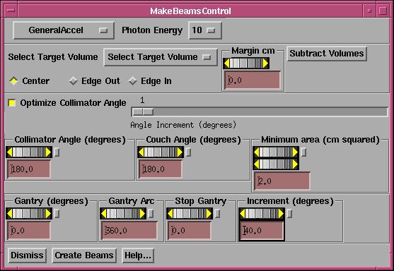
This function will generate static beams on a selected arc at selected intervals in degrees to conform to a selected target. You can set a margin for any volume selected. The margin refers to the margin of the volume, not the margin when the volume is projected to the beam's eye view plane.

For example, you might first generate beams every 40 degrees that conform to the prostate. Then you might generate beams every 40 degrees that conform to the prostate less the projection of the rectum. Then you can use the auto-weight feature to solve for the monitor units to use for each beam.

First select the treatment machine and then the energy desired.

Next select the target volume and the margin for that volume.

Hit the "Subtract Volumes" button to bring up a popup listing all outlined volumes for you to choose which volume whose projection you want to subtract. Note that you can select a separate margin for each of these volumes (positive margin means the margin is added to the volume, then its projection is subtracted). It would not make sense for you to select the target volume to be subtracted. The subtract volumes popup is described in the Beam section under the multi-leaf tool. However, here if the subtracted volume bisects the projected target into two or more pieces, a separate beam is made for each piece. For example, if the rectum in the AP direction bisects the prostate (target) into a left and right side, one beam will conform to the left side and another to the right side. Note that using the MLC control under the Beam toolbar this will not happen, a separate beam with a separate aperture is not made. But here multiple beams are made, each conformed to a separate projected piece of the target. Any further editing will require one to drag a leaf to a particular position.

You can select whether the leaf center is to touch the volume (we mean the projection of the volume), all of the leaf edge is to be outside of the target, or all of the leaf edge is to be inside the projected target volume (less all projections).

Leave the toggle button IN if you want to optimize on the collimator angle. You can set the increment for which collimator angles are tried. For example, if one, then every degree is tried. If set to five, then starting at the minimum angle, the increment is tried angles is five, for example, 0, 5, 10, 15, and so on. If optimizing on the collimator angle, the collimator angle set in the below control is ignored.

You can specify the minimum area in the beam's eye view plane at isocenter that the remaining projection is to have in order for a beam to be made. This projected area will include any added margin. If the projected area is less than that selected, the beam will not be made. If the projected area is zero, the beam is never made.

You can select the collimator angle and couch angle that all the generated beams are to have. As noted above, if optimizing on the collimator angle the collimator angle here is ignored.

Next you must specify the arc over which the beams are to be generated and the spacing in degrees between each generated static beam. Do this by selecting the angle at which the arc is to start, the direction and length of the arc, and the increment along the arc at which beams are to be generated. The generation of beams will stop if the next beam would go beyond the arc length.

For example, an arc length of 360 degrees starting at zero with an increment of 40 degrees would generate beams at 0, 40, 80, 120, 160, 200, 240, 280, and 320 degrees (0 or 360 is not duplicated).

Hit the "Create Beams" button when you have made all your selections. You can then select each beam to be edited, and look at the beam’s eye view for that beam to view the result for that beam.

Display Pull down

Under the Display pull down are options pertaining to displaying the plan. Because there may be more than one plan in the run of a program, the plans are not automatically displayed in frames. Rather you must select which frames to display the plans in. You can specify a specific frame or all the frames on the currently displayed screen. However, the program will not allow a plan to be displayed on an image that does not belong to either the primary stacked image set or on an image set not fused to the primary image set. A plan cannot be displayed in a frame in which a plan is all ready displayed. What is displayed are the beams, point doses, and isodose curves if also selected for display. Note that under the stacked image set pull down on the main you can redisplay an entire image set on a new screen, for the case you want to display a different plan on all the images of the same image set.

Display Plan Control Popup.

A popup tool is provided to remove a plan from being displayed in a frame. The same controls appear to display a plan but additional controls are provided to remove a plan from a frame or screen.

The central ray is drawn as a solid line to isocenter, and then drawn as a dashed line beyond. The beam’s eye view x, y, and z axes are drawn and marked. The z axis is the central ray, positive toward the source of x-rays, and lies coincident with the central ray. With the treatment machine pointed at the floor and the collimator unrotated, the x axis goes from left to right while standing in front of the treatment couch looking toward the gantry. The y axis is parallel to the long axis of the unrotated treatment couch and points toward the gantry. The origin is at isocenter. The intersection of the beam with the plane is shown. When the beam’s toolbar is actively selected, this area is tinted yellow.

There is an option to create a screen consisting of four frames, a transverse, coronal, and sagittal plane, and a 3d room view. The planes are either the center of the image set or may be the center of an outlined region of interest.

Evaluate Pull down

Items under the evaluate pull down have to do with calculating the dose and displaying the result. Because calculation times may be long, there is control to selectively select which frames the dose is to be displayed in. Each frame is calculated when it is selected here to display the dose. The hot spot in that frame will be displayed and marked with a star asterisk like figure.

Dose Matrix

Each beam maintains a dose matrix on diverging fan lines, the fan lines covering the area of the beam. A rotating beam would be simulated with multiple dose matrices at increments specified by the plan. The spacing between the fan lines and along the fan lines is specified by the plan, so that all the beams belonging to a plan use the same parameters. Each beam stores its matrix under its own subdirectory under the plan subdirectory. The matrices are written to disk files when the return button on the plan toolbar is activated.

For any two dimensional plane image displayed in a frame a two dimensional matrix will be generated that covers the entire image. The same spacing parameter specifies the distance between points. When the dose is calculated, the coordinates of each node of the two dimensional matrix is passed to each beam. The beam module will find the diverging box bounded by the fan lines that the point is inside. The eight corners of the box will be referred to when interpolating the dose at the position of the passed in point. Each beam will calculate the dose to each vertex of the diverging box on a need basis. When ever a reference is made to a vertex where the dose has yet to be computed, the dose is computed at that time. After calculating the dose to a plane, all the beams will have a swath through their dose matrices of calculated points. As more planes are computed, more of each beam’s dose matrix is computed. If any change is made to a particular beam, that beam’s matrix is reinitialized.

Likewise when a dose in a 3d perspective room view is computed, a rectangular array (lattice) of points is generated for the patient volume. Each of those points is likewise passed to each beam, so that after a room view display each beam will most likely have calculated the dose to all of the available vertices.

The Calculate All Beam 3D option will force all the beams to compute the dose to all the vertices on their respective dose matrices.

Calculation Matrix Spacing Control Popup

Calculation Matrix Spacing and Rotation Increment

A control is available to specify the spacing to use for all the dose matrices and the increment in rotation to simulate beam arcs. Making a change here will force all beams to dump their current dose matrices. The matrices covering planes and the matrix for room views also must be regenerated if a change in spacing is made here. The user will then have to reselect the frame to display the dose in.

The arc spacing is the increment to use to simulate an arc with fixed beams. This parameter is adjusted somewhat by each beam to fit the arc length of that beam so that the arc is simulated with equally spaced fixed beams.

Two Dimensional Isodose Control

2d Isodose Control

This control provides a tool for the user to specify the isodose value to be displayed. The dose may be displayed in cG or percent of dose to a normalization point (see Normalization Point under Options). Changing between cG or percent simply changes the label for the curves, the same dose is shown. The dose value desired is to be typed in the text field at the top of the popup. For special emphasis, you have the option to increase the width of any selected isodose line. The line width is in pixels and the default value is zero, which specifies the normal line width.

The isodose value may be tinted in a single color showing the boundaries and interior (higher doses) of that isodose line. You may use the mouse to select different isodose values to tint on the scrolled list below the text field for the value entry. Note also that the tint may be turned off and the tint color may be changed among the primary colors and additions of any two of the primary colors. Likewise any selected isodose line may be deleted or have its color changed. Colors are initially assigned at random. Note also that each isodose line has tick marks on the down hill side (lower dose) of the isodose line, analogous to topographical maps. The selected isodose lines apply to all 2d frames in which the dose has been selected to be displayed for the plan.

An issue that must be dealt with is what to do when two successive dose vertices span the skin boundary, so that one point is outside the patient and the next point is inside the patient. The plotting of the isodose line simply stops at that point. However, the tinted area necessarily requires a closed contour.

In those regions the tint follows a path between points inside the patient and outside the patient and does not accurately represent the dose.

Three Dimensional Isodose Control

3d Isodose Control Popup.

A three dimensional isodose surface may be shown in 3d perspective room views of the primary stacked image set or any image set fused to it. Only one surface can be shown at a time. The desired value is typed into the text field provided. Under the text field is a control for the transparency of the isodose surface.

Limitations apply here. A transparent surface can only be seen inside a second transparent surface if the inside transparent surface is drawn first. Two transparent surfaces that intersect will present a problem in that if surface A is drawn first and surface B is drawn second, then surface A can be seen inside surface B, but surface B cannot be seen inside surface A. This software will draw the transparent isodose surface before other transparent surfaces. No attempt is make to sort surfaces or part of surfaces. If this becomes a problem you have two options. One, make all the other surfaces opaque or make the isodose surface opaque. You can also use a cutting plane on volumes that are drawn. A second option is to display the isodose surface in wire frame. The wire, solid, off, control is below the transparency scale.

This control controls all frames simultaneously that show 3d room perspective views where the user has chosen to show the dose. The user must first choose to display the plan in the frame.

Specific Points

The plan does not have its own list of specific points. Rather, the only list of specific points is maintained by the primary stacked image set. Therefore all plans using the same stacked image set will calculate the dose to the same list of specific points. The controls for the specific points are under the Stacked Image Sets pull down on the main toolbar. Select Options and then Points.

However, we need the ability to specify the coordinates of a point in terms of the beam’s eye view coordinates of a specific beam. Therefore a control is provided here for adding a point where the position is initially specified in beam’s eye coordinates. The coordinates are then transformed to the stacked image set coordinates and the point is created and saved. The point is not moved if the beam is later moved. To delete a point use the above controls for points as described under the Stacked Image Sets Options. The beam’s eye view coordinate system is described elsewhere as well. In the unrotated collimator and gantry positions (beam pointed at floor), the x axis goes across the couch left to right when looking into the gantry, the y axis points toward the gantry along the gantry’s axis of rotation, and the z axis points toward the source of x-rays. The x and y axes rotate with the collimator.

Plan Points Toolbar.

Under the Evaluate pull down we have a points toolbar. Here the dose to the specific points may be computed, displayed, printed, or saved to a temporary file. We can select the popup to enter new points in beam’s eye view coordinates. There is also a mechanism for comparing measured to computed values for testing purposes.

Print Points

Simply hitting this button will cause the points to be computed and printed. However, the physics summary provides more information about points, such as their coordinates in plan and beam’s eye view coordinates, and the contribution of each beam to the point. The physics summary is printed from a print button on the dose prescription popup selected from the Options pull down on the plan toolbar.

File Points

Selecting this option, the point’s label and dose value will be written to a file in the temporary file directory where print jobs are also stored. The dose to the points are first computed. An example file follows:

// Test Square 12-Dec-2000-09:19:19(hr:min:sec)

// Label Dose in cGray

<* Example Label *> 1.299286

<* slice 10 row 4 column 7 *> 1.324436

The file is written in our ASCII standard whereby comment lines start with two slashes and are not read. The label for the point is enclosed between the <* and *> symbols. The dose value is simply a number set off by white space. This format will also be referred to below.

Display Point Dose

This choice will display the dose value computed for each point below the label for the point in all frames where the plan is displayed.

Point Dose Off

This will turn off the display of the dose value of the points. Note also that any change to the plan or a beam will also turn of the display of the dose values.

Add Point In BEV

Locate Points in BEV Coordinates Control

This tool is provided here as a convenience so that a point can be added to the stacked image set in reference to the beam’s eye view coordinates of a beam. The control is very much like the one provided by the stacked image set under Options, Points toolbar. However, we have added an option menu to select the beam. Below the option menu are controls for the x, y, and z coordinates of the point. The point may not be located with the mouse. Do that on the control provided by the stacked image set. This control is provided for the case when a point must be specified in relationship to the coordinate system of a beam. Likewise, to delete or otherwise edit points, use the other controls provided by the Stacked Image Sets Options.

Compare to Measured

This option was provided for a very narrow purpose. Specifically, we irradiated a Rando Phantom and measured the dose at specific points and wanted to be able to display the measured value with the computed value. The measured values must be written to a file in the same format as the computed points are written to as described above. Selection of this option will prompt you to enter the file name of the measured points. The measured points are associated with the computed points by means of the point’s label. The labels are not directly compared. First each label is converted to lower case and then all spaces are removed and then compared. Care must be taken that the labels will remain unique when the user creates the labels. For a match, the measured value will be displayed below the computed value. An m is also appended to the measured dose value. In our use of the Rando Phantom we labeled the holes according to a scheme. There are 7 rows and 13 columns of holes with the 3 cm matrix drilling. Each hole is known by its slice number, row number, and column number. By labeling the holes consistently, the measured values can be matched up with the computed values and displayed. The specific points are also computed upon selecting this option.

We have also written a program that will compare measured and computed values, CompareRandoPoints. Invoke this program and on the command line provide the name of the file that contains the measured points, the name of the file that contains the computed points, and the name of a file to write the report to. This program assumes that only numbers appear in the label field, consisting of the slice number, row number, and column number separated by spaces and sorts values by those indices.

This labeling scheme could cause some confusion in the above display function in frames as 11 1 1 would be indistinguishable from 1 1 11, for example, after removing spaces. The row number is only in the range of 1 to 7 and the column goes only from 1 to 13. Use leading zeros for the slice number and column number for single digits if there is a possibility of confusion, i.e. 11, 1 01 and 01 1 11.

Plan Options Pull Down

Dose Prescription and Normalization Point

Dose Prescription and Normalization Control Popup.

On the options pull down we can select the dose prescription method. Because the dose prescription might be in terms of the dose to the normalization point, we put both controls on the same popup.

Show Dose or Percent

In the upper left hand corner of the popup, you can select to show either dose in centiGray, or percent of dose. The default is to show dose. To show percent, hit the percent choice. BUT, percent of what? To the right of the show dose or percent area is where you can select the normalization point. When you show percent, it will be the percent of this point. Changing between dose and percent simply changes the labels for the same selected isodose lines.

Normalization

Here we specify where the normalization point is.

The left choice is to normalize to the isocenter of a particular beam. Below the choice you pick the beam. If all beams have the same isocenter location, it won't make any difference which beam you choose.

The middle choice is to normalize to the nominal dmax point of a particular beam. Here the point will be on the central axis at the depth of the nominal dmax depth, for example 1.5 cm if 6x. The same option menu selects which beam is to supply the dmax point.

The right choice is to select some specific point for the normalization point. This is a point that you locate within the stacked image set under the Stacked Image Sets pull down on the main tool bar, to Options, to the Points toolbar. The option menu below Specific Point on the right is to select which point among the list of points.

Prescription

The dose prescription method is selected here. There are three choices: specify the dose to a point for each beam, specify the monitor units for each beam, or specify the dose to the normalization point and then select the weight for each beam.

Dose to a Point

For each beam, you must specify the dose that the beam is to give to some point. Lengthen the popup or scroll to each beam control area. You type in the dose to the beam's point. This entry also determines the relative weight of each beam. Below the type in area, you specify what is to be the beam's point. The choices are identical to the normalization point controls above. You may select the isocenter or dmax point of any beam. The default is the beam's own isocenter point. Or you may pick a dmax point of a beam or lastly, a specific point located from the stacked image set.

After specifying the dose and dose point for each beam, hit the Apply button and the monitor units will be displayed for each beam. You will notice a slight change in the dose values. This is because the dose is shown for the monitor units rounded off to a whole number. Under dose to a point, you cannot specify the monitor units. Monitor units are computed when the Apply button is hit.

Monitor Units

Choose this option to specify the monitor units each beam is to get. You must type in the monitor units for each beam. Then hit the Apply button and the dose to each beam's point will be shown. The monitor units used with the open field and wedged field is also shown. If a wedge is present and an open field and wedged field are being mixed to make a smaller wedge angle, you will see the respective monitor units for the open and wedged field. You cannot change that here. You must set the wedge angle under the wedge option for each beam to less than the nominal wedge angle to mix open and wedged fields and set the ratio.

The dose to each beam's point is displayed when the Apply button is hit.

Dose to Normalization Point

Choose this option to specify the dose that the normalization point is to get. Then select the percent. For example, 180 cG and 95% means that 95% of the dose to the normalization point will be 180 cG. Under this option you specify the weight of each beam by typing in the numbers for Dose or Weight for each beam. Here the entry is now weight. This is the relative dose each beam is to give to its weight point relative to the other beam's weight point. Hitting the Apply button will display the monitor units and calculate the actual dose to each beam's weight point.

The monitor units are computed and the dose to each beam's point is displayed when the Apply button is hit. You can then select to redisplay isodose curves to see how a change in weight affects the dose distribution.

Print Physics Summary

A physics summary is printed when the print button is hit. Note that the physics summary contains a plan ID number. If any change is made to the plan that effects the dose, the plan ID is incremented. The plan ID is also displayed on all the 2d and 3d frames where the plan is displayed. This ID number serves as a control to guarantee that a print out belongs with a particular screen print. This print out contains information about each beam and the dose to specific points, and should be placed in the patient’s chart and used as the definitive document for the plan.

Auto Weight

The function will compute the monitor units for each beam given a minimum dose constraint on a target volume. The dose to other outlined regions of interest can be minimized or constraints imposed.

The beam auto weight toolbar.

This toolbar provides tools for solving for the monitor units for each active beam in an optimal fashion. Four different optimization schemes are supplied:

(1) linear programming solved with the Simplex method,

(2) a down hill search method with penalties added to the objective function for violated constraints.

(3) the Cimmino algorithm,

(4) Simulated Annealing.

The behavior of these four solution methods are different and effect the way you must set up the problem in choosing parameters for targets and organs at risk (OARs).

Plans must be evaluated for the correct dose and dose distribution after running this algorithm. You cannot assume this algorithm will find the correct monitor units for all the beams. You must evaluated the plan as you would any plan when changing beam weights.

Beams

By specifying different apertures for different beams, including beams with different apertures for the same beam location, you can achieve plans meeting difficult treatment plan specifications. We recommend that you read the reference:

"An Optimized Forward-Planning Technique for Intensity Modulated Radiation Therapy" by Y.Xiao et. al, in Medical Physics, Vol. 27, No. 9, Sept. 2000, pages 2093-2099,

as to how to achieve similar results to intensity modulated radiation therapy (IMRT) with this method. Two or more beams at the same coordinates but with different field shapes results in some intensity modulation, so in some respects one could call this IMRT. Our definition of IMRT is the division of a beam field into pixels and solving for the intensities of each of those pixels separately, often referred to as inverse planning. We are not doing that here, but we can achieve similar results here with what is usually referred to as forward planning. The beams and beam shapes are predefined as normally done in planning. This tool is used here to help find the monitor units to use for each of those beams to achieve a clinical end. Below we only have constraints on dose, we do not deal with volume histogram constraints.

The Simplex method has a linear objective function and linear constraints. It has the advantage of strictly enforcing constraints and reporting if a feasible solution (a solution that satisfies all the constraints) is not possible. The down hill search method and simulated annealing method have only an objective function and use the same objective function. Constraints are folded into the objective function by added a penalty to the objective function if a constraint is violated and so will return a solution even if the constraints cannot be all satisfied, with the solution being a compromise. The down hill search could get trapped in a local minimum if there are multiple minimums. The simulated annealing algorithm might be more likely to find a global minimum. The Cimmino algorithm only has constraints and has no objective function. It is described in the above reference. If all the constraints cannot be satisfied, a compromise solution is returned.

Select Target and OAR

All three algorithms use the parameters you define or select with the Select OAR and Target popup, but they will use those parameters differently. On this popup you can select which volume is to be the target volume. You must specify a minimum dose for the target. You can optionally specify a maximum dose as a constraint. Notice that there is also an importance parameter and a penalty parameter.

You may also select volumes as an OAR. You would not specify a minimum dose for an OAR, but you might specify a maximum dose as an optional constraint. The importance parameter and penalty parameter might also apply depending upon the algorithm used. How the constraints, importance value, and penalty value are used depends upon the algorithm selected to solve for the beam weights (monitor units).

Select target and OAR popup tool.

NOTE: A blank text field for an upper constraint (maximum dose) means there is not an upper constraint. Whereas a value of zero creates an upper constraint of zero dose.

The contibution of a volume to the objective functions are normalized by the number of points in the volume so that a large volume does not dominate.

The Simplex Method for Linear Programming

The simplex method solves for linear objective functions and linear constraints. All our constraints are linear in that the dose is specified as being either above some selected value or below some selected value. The program minimizes the sum of the dose to the target and OARs.

The linear sum of dose in the objective function means that our clinical objectives may not be automatically met when this sum is minimized. For example, if two points each get 90 cG the sum is 180, but if instead one point were to get 0 and the second to get 180, the sum is still 180. This is different from taking the squares of the dose. Taking the squares the 90, 90 situation, i.e. 2 times 90 squared, results in an objective function value of 16,200 and has a lower value than the 0, 180 situation, where 0 squared plus 180 squared results in a value of 32,400. Therefore a linear sum does not distinguish between all the dose being concentrated in an area from the same dose being spread out. For example, for a four field box on a pelvis, this algorithm is probably going to pick the A/P fields over the laterals because the A/P thickness is typically less than the lateral thickness. But clinically, we want the dose spread out outside of the target and not concentrated. However, minimizing the sum of the dose with a floor on the dose enforced for the target will push the solution toward a uniform dose in the target.

To force the simplex method to spread the dose out among all the fields will probably require an upper constraint on the dose to the body outside the target. To achieve this, make a new volume from the target with an added margin of 2 to 4 cm (use the function under Volumes on the Contouring toolbar called New Volume From Old). Then create yet another volume that is the skin boundary with this target plus margin volume subtracted. Put an upper constraint on this volume. Start with the target dose and run a solution. Then lower the dose. You can do this quickly using a binary search where you half the difference, i.e., set as the upper constraint the target dose divided by two. If there is no feasible solution take the dose midway between the infeasible solution dose and the last dose that you did get a feasible solution. With a few trys you will arrive at a good solution.

With the simplex method, the importance value that you can specify for a volume simply multiplies the dose by that value and adds the result to the object function that is being minimized. The objective function is the sum of the dose to all points inside the target volume and the sum of the dose to all points inside OARs (but multiplied by the importance value for that OAR or target). The penalty value is not used. The dose to all points in the target volume is constrained to be greater than or equal to the target dose specified for that volume. An upper dose constraint is optional for target volumes. An upper constraint is also optional for OARs.

Any time you specify an upper constraint, a feasible solution that satisfies all the constraints may not exist, and the simplex method will report if a feasible solution does not exist. You will than have to raise an upper constraint. That is why it is best that you start with a large upper constraint for which you can get a feasible solution and then lower the constraint until a feasible solution does not exist.

Cimmino Algorithm

For a reference see:

"On the use of Cimmino's simultaneous projections method for computing a solution of the inverse problem in radiation therapy treatment planning" by Yair Censor, Martin D. Altschuler, and William D. Powlis in Inverse Problems Vol 4, 1988, pages 607-623.

and

"An optimized forward-planning technique for intensity modulated radiation therapy" by Xiao et. al., Medical Physics, Vol 27 No 9, Sept. 2000, pp. 2093-2099, particularly pages 2094-2095.

There is no objective function to minimize or maximize. This algorithm simply finds a solution to satisfy all inequalities or a compromise if a feasible solution is not possible.

A selected OAR will be ignored unless you specify an upper constraint value. The value could be zero (the field must have a number in it and not be blank).

The importance value weights each selected volume, the larger the importance the more the weight. The weight is divided by the number of points in the volume. The penalty value is ignored.

We would suggest you first select the target and the minimum target dose. Then select OAR's and set the upper dose to zero. If there is no upper dose limit set for an OAR, the OAR is not considered. The Cimmino algorithm only has constraints, there is no objective function to minimize. But the constraints are weighted according to their importance. To cover the target, you may have to increase its importance value.

The Cimmino algorithm stops when either the solution distance is no longer changing, or the maximum number of iterations is exceeded. You can change either of those two parameters. The distance is in the units of monitor units. But the algorithm considers the weight in moving a vector so the distance is divided by the total weight.

Cimmino Set Parameters Popup

Making the stop distance smaller will make the algorithm run longer, and increasing the iteration limit will permit the algorithm to run longer. Trial and error is required to adjust these parameters and see how they might effect the solution. But we have picked default values that should work in most cases.

Down Hill Search with Penalty

The down hill search method simply searches to minimizes an objective function. [The simulated annealing algorithm uses the same objective function.] Constraints are not enforced as there are no constraints in the algorithm. Rather, constraints get folded into the objective function.

For the target dose lower constraint, the contribution to the objective function is the difference between the dose and minimum target dose squared, and then multiplied by the importance value. The penalty value is then added only if the dose is less than the target dose. The contribution is then divided by the number of points in the volume.

For any volume with an upper constraint, the target or OAR, there is only a contribution to the objective function if the dose exceeds the upper constaint value. The contribution is the penalty value multiplied by the importance value and divided by the number of points in the volume.

For all OARs, the dose is squared and multiplied by the importance value and divided by the number of points in the volume. The penalty value is not used.

This is called non-linear optimization because the objective function is not a linear equation. The algorithm should find a feasible solution if one exist because the cost will be lower (the cost being the value of the objective function) for a feasible solution. Remember that a feasible solution is one that satisfies all the constraints. However, it might be possible for a local minimum to exist in an infeasible region. And if there is no feasible solution, a compromise is found in that the objective function is minimized.

After selecting your targets and OARs, you can always hit the Simplex solution button first to find out if a feasible solution exist. If there are no upper constraints there will always be a feasible solution, since you can always make the monitor units large enough to cover the target dose. The exception might be if the beams do not irradiate the target.

For the down hill search we suggest you first try simply selecting a target, specify the target dose, and select the OARs, one of which might be the entire body.

Simulated Annealing

The simulated annealing method uses the same objective function used by the down hill search method described above. The user can control the cooling schedule. A longer cooling schedule takes longer but improves the chances for finding a good solution.

A reference is:

“Optimization by Simulated Annealing” by S. Kirkpatrick, C.D. Gelatt, M.P. Vecchi, Science, Vol. 220, No. 4598, pp. 671-680.

Simulated Annealing Stop Parameters

The algorithm generates monitor units for each beam at random. The standard deviation of the spread of these monitor units is decreased as the algorithm runs. The square root of the variance is the standard deviation. The standard deviation is incrementally decreased when the number of iterations per step has occurred. This is set to ten in the above example (the default value). After every ten iterations, a sum that starts with zero is increment by the increment value (0.01 in the above example, the default value). The negative of this sum is the argument to the exponential function, e raised to the –sum, i.e., exp(-sum). This term is the standard deviation fraction:

Sd_fraction = exp ( - sum)

Thus the value of the exponential function, sd_fraction, starts at one and decreases to zero. The standard deviation is this exponential function value times the initial standard deviation. The algorithm stops when the standard deviation is less then a minimum value, currently 0.5 monitor units.

These details are not necessary for you to know. Just that making the increment smaller or making the number of iterations per increment larger will cause the algorithm to run longer, and will increase the chance of finding a good solution.

The same cooling schedule is used to compute the probability of accepting an increase in objection function. The variance of the objective function is periodically computed. The probability of accepting an increase in objective function value decreases according to the same exponential function. The probability of keeping an increase in cost is computed by:

Probability = exp( - 0.5 * variance) * sd_fraction

Where variance is the current variance of the objective function, and sd_fraction is as above. Note that the above exponential is the Gauss function or normal probability distribution. The best solution seen is what is returned.

Using the Toolbar

Once you have selected the target and OARs and call for a solution, the program must compute the dose rate each beam contributes to each point. A distribution of points are found in each volume to represent that volume. This dose calculation can take a few minutes, but the results are saved and you can change optimization parameters and call for a second solution without the points having to be recomputed. Only if you change a beam or add a new volume will the calculation of dose have to be repeated. You can therefore try different parameters and look at the solution. The monitor units found with each solution will be displayed to you and automatically installed for each beam.

Output Plan

The plan can be output to an accelerator in two formats: Dicom RT and Elekta’s Transa format.

Dicom RT

For Dicom RT you just select this option and the plan will be written to a file in the temporary directory where print jobs get written (see file tmp.dir.loc in the program resources directory identified in your current directory by rlresources.dir.loc, see the System 2100 manual). A popup will inform you of the file name created. This file will contain all the beam coordinates, monitor units, energy, wedge, and multi-leaf information. [You can use program DicomRTDump to display the information in a Dicom RT file.] To send this file to a linear accelerator you will have to use a third party Dicom communications package, of which there are apparently many choices.

Elekta Transa

Elekta (formally Phillips) has a private protocol for transferring beam shapes to their multi-leaf collimator. Only the energy, field shape, jaw setting, collimator angle, and multi-leaf positions can be written out. The files get written to a directory and the linear accelerator does an NFS (Network File Sharing) mount of that directory. In the machine’s data directory must be the file ElektaTransa.loc. An example of the file follows:

// Directory where plans are to be exported to. The program

// first looks into the machine's beam data directory.

// If there it is read there. If not found it looks into the

// program resources directory.

/* file format version this file */ 1

/home/export.d/patients

/* limit of number of plans per patient directory */ 3

/* limit of number of beams per plan */ 8

/* name of machine to put in the file */ MLC_01

/* number of characters of patient dept. id # to use */ 7

/* number of characters of last name of patient to use */ 3

/* number of characters of first name of patient to use */ 0

/* number of characters of middle name of patient to use */ 0

This file specifies the directory where the beam data files are to be written to. The directory specified here must be listed in the /etc/exports file. In that file one list the directory, as above, and then possibly the host names of systems the directory may be exported to. If no names are listed the directory can be exported to any system. For example:

/home/export.d/patients MLC_01

will allow the directory /home/export.d/patients to be mounted by the system with host name MLC_01.

It is necessary that read and write permission be given to everyone for this directory, and all components of the path must exist. To give read and write permission the command is:

chmod ugo+rw /home/export.d/patients

NFS must be running on the treatment planning computer. For more information see the Elekta Precise Treatment System External Interfaces Manual, TRANSA.

The machine name must be that which the accelerator identifies itself for this purpose.

The program must build a patient ID. The ID is actually limited to 14 characters. Specifying more characters in the above file will not cause the program to run over the 14 characters. In the above example, a patient ID is built from the first 7 characters of the department number and the first three characters of the patient’s last name. Only 12 characters are actually used in any case. A number is appended if the number of sites should exceed 3. In the above example, if there are in fact 26 beams in the plan, a second patient ID will be created to hold the last two beams. The limit on the number of beams per site and sites per patient ID is a specification from Elekta.