Contrast and Edge Enhancement

To adjust the contrast of an image, hit the Contrast button on the right hand corner of the screen. The preferred visual model for CT scans to use is 12 planes as the contrast can be changed quickly by reloading the look up table. For an 8 or 24 plane visual, the image must be reloaded for each contrast change. The action will therefore be slightly different depending upon the visual model for the window.

For 12 plane visual, the first 8 planes are normally used to display the gray scale. Here in the representation of the binary value of a pixel, each bit occupies one plane. One can count from 0 to 255 with eight planes. The next 3 planes are used to display colors. The top plane is used for an overlay color, used when outlining for example. When contrast is selected, the present image is converted to occupy all 12 planes and the look up table is reloaded so that the same contrast is displayed for the image. With 12 bit planes one can count from 0 to 4095. But at each address is stored the intensity of red, green, and blue each with an intensity of from 0 to 255. As the contrast width and center slider is moved, the look up table is reloaded. Because on Silicon Graphics computers there is only one 12 plane look up table, the other frames will be observed to change. The change will be mainly to dark because on a scale of 0 to 4095 those images have pixel values of 0 to 255. In the frame selected, contoured colored lines will be interpreted to have a gray color. When the Done button is hit on the Contrast popup, the image is recomputed to occupy 8 bits but to show the same contrast, with the look up table correspondingly loaded to simply count from an intensity of 0 to 255 for each of red, green, and blue, for the first 8 bits.

With an 8 or 24 plane visual, the look up table is not reloaded. Therefore the other frames will not change in appearance. However, the contrast of the frame under adjustment will not change while dragging the contrast width and center sliders. Rather, the image will be reloaded when you release the slider.

For other images, the contrast range scales will adjust themselves to accommodate the range of pixel values, up to 16 bits (0 to 65535).

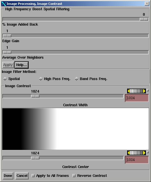
Edge Enhancement

Here we can amplify high spatial frequencies with a spatial filter, high pass frequency filter, or band pass filter. These tools can be used to enhance the edges of an image. This might be useful in a CT scan that includes lung, where one wants to bring out the structure inside the lungs, and still see details elsewhere without washing out the rest of the image.

Spatial Filtering for Edge Enhancement

First we low pass the image by replacing each pixel with an average over an area. The size of the area is determined from the "Average Over Neighbors" parameters. If the value is one then the area is a 3x3 matrix with the pixel at the center. If 2 then the matrix is 5x5, and in general the side of the matrix is one plus two times the value. As this value is increased, the computation times increases. For small matrix sizes, such as a 3x3 matrix, the spatial filter will compute faster than doing frequency filtering with the Fast Fourier Transform making use of the convolution theorem.

The program then computes the value:

edge_gain x [ pixel_value - average pixel_value ]

% Image Added Back

--------------------------- x pixel_value

100

To this is added a percent of the original pixel value:

And then we shift the gray scale relative to a nominal pixel value of 1024 by adding in the below term so that the contrast window does not need to be moved as much as it would otherwise:

100 - % Image Added Back

---------------------------------- x 1024

100

The final equation is:

100 - % Image Added Back

---------------------------------- x [ 1024 - pixel_value] + pixel_value +

100

edge_gain x [ pixel_value - average pixel_value ]

The resulting image data is shifted so that the most negative number is shifted to zero. The range will be rescaled in need be to stay in the range of a 16 bit number.

For a discussion of high boost filtering, see the book Digital Image Processing by Rafael Gonzalez and Richard Woods, Addison-Wesley Publishing Co. (ISBN 0-201-50803-6), pages 195-197.

Another reference would be pages 114-117 of the book from the Proceedings of the 1997 AAPM Summer School: The Expanding Role of Medical Physics in Diagnostic Imaging.

We suggest that you leave the Average Over Neighbors slider at a value of one, and try an edge gain greater than zero and then adjust % Image Added Back. You may have to play with all the values to get what may be useful to you.

If the Edge Gain is zero, then the spatial filtering is not performed.

High Pass and Band Pass Frequency Filtering

You also accomplish frequency filtering. By this is meant transforming the image into the frequency domain, multiplying by a filter function, and then transforming back. Only one filter function is provided, a Gaussian curve. For a high pass filter, the curve, once reaching the value of 1.0 continues on so to the highest frequency. The highest frequency is the Nyquist frequency = 0.5/pixel_size where pixel size is the pixel size of the image. You can control the width and center of the Gaussian curve (width computed at ½). In addition you can add a floor to the filter function, with the Gaussian ranging from the floor to a value of 1.0.

An analogy you can think of is a piano. A filter would be something that would amplify the sound from each key separately. High boost would amplify the notes from the right side of the keyboard more then from the left side (which is lower frequencies). A filter function would be the amplitude plotted from left to right for each key. The keys increase in frequency from left to right.

Images also are the summation of frequencies, which is the rapidity of the transition from black to white. A smooth slow transition would be a low frequency. A sharp edge requires a high frequency. These frequencies are two dimensional.

You can specify a frequency response for filtering an image. The filter is drawn on top of the contrast display shown below. Zero frequency is at the left, the highest is at the right. The highest frequency in an image is 0.5 X 1.0/(the pixel size), which is called the Nyquist cutoff frequency.

A Gaussian curve is here provided for a frequency filter. You can adjust the width of the curve and center. For a high pass filter, the maximum amplitude is simply continued.

There is also a floor control, to add in lower frequencies.

The high pass filter function is thus:

A + [1 - A exp( -h² (r-c)²) ] for r <= c

F(r) =

1.0 for r > c

where A is the floor, low pass gain, 0 to 1, and h = 1.665109222/width.

The width computed for a value of 1/2 of the Gaussian.

r is the radial spatial frequency in cycles/cm.

For the band pass filter, the down side of the Gaussian is also used.

The fast Fourier transform is used to convert the image, the filter function is multiplied, and then the image transformed back. The image data is shifted so that the most negative number is zero, and will be scaled if need be to remain in the range of a 16 bit integer.

You will have to readjust the contrast settings after the transformations. Adjust the filter parameters and then hit the Apply button. If the range of the image data is not changed, the contrast settings are left as before.

Shown below is the contrast tool configured for the band pass filter.

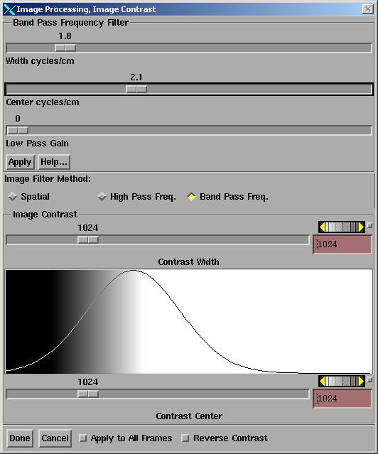
Note that the frequency filter is plotted on top of the contrast image, ranging from zero special frequency on the left to the Nyquist on the right. You have to hit the apply button to process the image in the current frame.

Unselecting any of the three image processing methods will restore the image to an unfiltered state.

Zooming

Zooming is performed by first selecting the frame and then clicking the middle mouse in the frame. Use the right mouse button to zoom back out.

Creating a New Screen

Hit the Screen Control button on the right lower side of the screen. On the popup select New Screen. Then select the number of frames that you want either by hitting one of the pre-defined buttons or typing in the number of rows and columns. If you select more rows than columns, the frames will appear in a scrolled window. For your convenience be sure to add a name to the screen in the text field. Any frame in a screen that you create can have its contents later deleted.

Screen Control Popup

Reconfiguring an Existing Screen

Hit the Screen Control button and then select the Change Screen Layout button. You can specify the number of columns and the program will compute the number of rows needed to hold all the frames. You can increase the number of frames by typing in a larger number of columns. You will not be able to reduce the number of frames that are actively being used. The program may override your choice of number of rows to hold the present number of frames used on the present screen. If there are more rows than columns, the frames will appear in a scrolled window.

Screens that hold a stacked image set are fixed in the user of the frames. You may not delete a frame (unless deleting an image from the stacked image set) and you may not use any frames left over.

Display of Stacked Image Set Images

The image is shown with coordinate information in the upper left hand corner of the image. You may have to maximize an image to full screen to see the coordinates. The first number top left is the frame number. Next follows the normal vector in IEC coordinates. To the right of that is the coordinates of the center of the image in centimeters in IEC coordinates. The origin is the center of the stacked image set. Below on the next line is the angles for the normal vector in the order of theta, phi, twist.

Selecting Stacked Image Set Images

There are two ways you can copy an image from the image set to an unoccupied frame on a screen that you have created. One is to use the Copy, Move, Image Plane under the Stacked Image Sets pull down on the main menu, and the other is to use Select Image From Set also under Stacked Image Sets. With the latter, you will see a scrolled list of all the images. Shown will be the IEC coordinates of the center of the image, and the coordinates of the image assigned by the imaging system. For Dicom, the imaging system coordinates are for the upper left hand corner of the image.

Select an Image from the Stacked Image Set Popup for Display

Select an empty frame you want to put the image into by clicking the mouse on the button that occupies the frame. Then select the image from the list of images. You can continue to select different frames and images while the popup is up.

Reformatting Images from a Stacked Image Set

Go under the Stacked Image Sets pulldown on the main tool bar to Select Image Plane. You will then select one among Transverse, Coronal, or Sagittal as a starting specification. However, you can change this on the popup that comes up. All images in a stacked image set are in effect reformatted images. The plane within the stacked image set is specified and the image data is filled in pixel by pixel. The images of the stacked image set are displayed by specifying the plane that the image occupies. Specifying other planes will cause the pixel values to be filled from the stacked image set. If a pixel falls between two images of the stacked image set, the pixel value can be interpolated between the two images. Be aware that the interpolation is along the line perpendicular to the stacked images. This applies even if the images are all leaning as they would for CT scans taken with a non-zero gantry angle.

Reformat Image Popup

Note that on the popup there is an option menu for choosing the image set.

The slider that is perpendicular to the image plane type selected among transverse, coronal, and sagittal will be shown in a different color. The computed scouts for the image set will be shown at the bottom of the popup, unless there was only one image in the image set. As a slider is moved, the intersection of the plane specification with each scout view is shown. Bare in mind that the computed scout views occupy planes that are through the center of the box containing all the images in the stacked image set.

To display the image in the selected plane, click the mouse on an empty frame and hit the Apply or Done button. Note that interpolation may be turned or off before depositing the plane specifications in the empty frame. By default interpolation is on.

You may also view the intersection of the plane with any image presently displayed in the selected image set. Use this option if you want the image to go through some point that you can see on another image. To do so select the Draw in All Screens toggle button. You will also have to select a screen in which images of the image set are displayed. If the drawing slows down the slider too much, you can select to turn off drawing with the drag of the slider. The drawing will than only occur when you release the slider after moving it.

The Rotation button is provided on the popup to allow you to rotate the selected plane. Pushing the Rotation button will bring up an additional popup. On this popup will be shown a wire frame view of the IEC coordinate system in green marked with X, Y, Z, and the viewing coordinate system in red marked with v, v, w. You eye is looking down the w axis with the u axis horizontal.

Reformat Image Rotation Control Popup

The angles phi and theta are specified in spherical coordinates, with theta rotation around the Z axis measured from the X axis, and phi rotation from the Z axis. Twist is rotation around the w axis. Any point of view can be selected with these three angles. Note, however, that a given point of view dose not have a unique set of angle coordinates.

Given a point of view, you may also slide the plane specification along the w axis by adjusting the w vector offset scale.

For each of the coordinates where is a coarse slider or thumb wheel, a fine thumb wheel, and a type in text field. Note also that the wire frame view is a 3d room view window and includes its own thumb wheels for selecting a point of view of the wire frame display.

An Apply button is also supplied with the Rotate popup for depositing the plane specification in a frame.

Reformatting an Image Set

Under the Stacked Image Sets pulldown is Reformat Image Set. This control may be used to reformat in equal increments images from the image set in parallel transverse, coronal, or sagittal planes. The range may be selected over which the image set may be reformatted. For example, if one selects Coronal plane type, the bordering lines will be shown on the scout views provided with the popup. The minimum and maximum range controls may be adjusted to specify the boundaries within the image set where the images are to be generated. A spacing control is also provided.

Reformat Image Set popup control.

Given the boundaries of the selected range, the center is found. Then image planes are generated toward the maximum and minimum boundaries. The last plane within the range is what is drawn on the scout views. Because of this you will notice the range lines moving slightly as the spacing is changed. Nor will the minimum and maximum range lines appearly to move smoothly as you adjust the controls because the last plane position within the range is what is shown. A screen name may be optionally assigned. Upon hitting the OK button, a new screen is created and the image planes are generated with the image data reformatted to fill in the planes.

Selecting Other Images for Display

This topic was covered above in the chapter on Other Images.

Copying Images

Copy Move Image Plane Popup

Copy from same image set

We do not copy images, we copy the plane specification within the image set and copy that plane specification to another frame. All images in a stacked image set are reformatted images, with the stacked image set filling in the pixel values. If you want to display an image again that is not in a stacked image set, simply reselect that image again for display in a different frame (see the chapter on Other Images).

Under the Stacked Image Sets pulldown in the main menu, select Copy, Move, Image Plane. A popup will appear. At the top of the popup select the stacked image set. Click the mouse on the frame containing the image plane of the image set that you want to copy. That image will reappear in the popup. Use the Copy To Frame button to copy the plane specification to some frame that you have selected.

Copy between stacked image sets

This function can also be used to specify the same plane, relative to the patient, in a different stacked image set. The plane specification is copied from the frame where the mouse is clicked. The image data comes from the stacked image set that is selected at the top of the popup. The plane specification is copied to the frame when the Copy To Frame button is hit for the image set that is selected. That image set will appear in the frame selected.

Interpolate

In both of the above cases, interpolation of pixels can be turned on or off. Interpolation would occur if a pixel in the image plane falls between two images in the stacked image set. By default interpolation is on.

Contrast

Note that the contrast of the image shown in the popup can be adjusted with the button provided on the popup. The contrast button on the main screen will only work for frames selected on a screen.

Saving a Frame

You can save the image configuration for an image from a stacked image set by saving the frame. Go to Save Frame under the Frame pulldown menu. The program will require you to input a unique file name. What is saved is the plane in the image set, the contrast and edge enhancement settings, and any zoom factor. This information is saved under the image set directory. You will have to read in the image set to restore the frame saved for an image set. Note that this funciton also saves the configuration for 3d room perspective views of the image set. To restore a frame, you must click the mouse on an empty frame that is on a screen that you created. Then choose Restore Frame in the Frame pulldown menu. You will have to pick the image set and then choose the file name that the frame was saved under.

Comparing Images

Compare Images - Checkerboard

Checkerboard Compare Images

This feature will allow you to create a checker board pattern, with the two images alternating every other square. This may be useful for judging the goodness of a solution for fusion between a CT and an MRI image set. Go under Images in the main tool bar to Compare Images - Checkerboard. Two popups will appear. One will hold the image and the other a control area. To get the first image click the mouse on any frame that has a 2d image. Click the mouse on any other frame that has the other image you want to compare to.

Control for the CheckerBoard Image Compare

In the control area you can adjust the contrast of each image independently of the other. You can also change the size and number of the squares and move the squares sideways and up and down. This last option is useful for moving the boundary between the two images.

Use the Copy To Frame button to copy the image in the popup to a frame that is on a screen. Note that a control button will appear that will allow you to bring up the control panel again for the checkerboard pattern. The contrast button on the bottom right of the screen will not work with these frames (since there are two images mixed together). The contrast of each image must be adjusted using the control panel.

Compare Images - Color Mix

Select this feature under Images on the main toolbar. Like the checker board tool above, you click the left mouse on each frame that contains one of the two images that you want to compare. Three color mix choices are available:

Control for the Colormix Image Compare

green-magenta, blue-yellow, and red-cyan. For example, one image is displayed in green and the other in magenta. Each of the two color pairs adds to white, so that images with the same gray scale component on a particular pixel will show white. This tool is useful for testing the goodness of image fusion between two CT scan image set. You can adjust the contrast of each image separately. You use the Copy to Frame button to copy the two images to an empty frame. A control button is created in the lower left hand corner to bring back up the control panel.

Add Images

This feature allows you to add two images together. However, no controls are available to move one image in relationship to the other. The weight of the two images added together may be adjusted. The pixel values are added after the image is put through the contrast window. The final pixel value shown is given by:

pixel value = [ (100-weight2) * pixel_1 + weight2 * pixel_2 ] / 100

Add Images control popup.

where:

weight2 is the weight for image 2,

(100-weight2) is therefore the weight for image 1, pixel_1 is the pixel value from image 1 after contrast is applied, pixel_2 is the pixel value from image 2 after contrast is applied.

Simply click the mouse on two successive images to be added together.

Difference Images

This feature is similar to add images above, except here the difference between pixel values is taken. Because we cannot display a negative pixel value the absolute value of the result is displayed:

pixel value = Times_factor *

abs[ (100-weight2) * pixel_1 - weight2 * pixel_2 ] / 100

pixel value = min(255, pixel value)

where:

weight2 is the weight for image 2,

Times_factor is a multiplication factor,

(100-weight2) is therefore the weight for image 1,

pixel_1 is the pixel value from image 1 after contrast is applied,

pixel_2 is the pixel value from image 2 after contrast is applied.

Difference Images control popup.

Note that the absolute value is taken of the difference in pixel values, and then the result is multiplied by the times factor selected on the slider below the weight 2 slider.