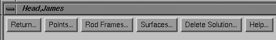
An Example: CT head to MRI head
Image Fusion
|
Select image sets to fuse toolbar |
You
can fuse any two stacked image sets. By
fusion, we mean solving for a rigid transformation from the patient anatomy in
one image set to the same anatomy in the other image set. You can use the result to display the same
plane in the patient in each image set.
|
Select image fushion method toolbar |
To
accomplish image fusion there must be something in common between the two image
sets that can form the basis of establishing the relationship between the two
image sets. We have provided three
separate tools for solving for the transformation between two image sets:
(1) If at least three distinct common points can
be identified in each image set, the best fit of the transformation between the
two sets of points can be solved for.
(2) If the patient had a common stereotactic
frame system on for both image sets such that the anatomy is located
identically relative to the respective stereotactic coordinates, then locating
the frame systems will provide a solution for image fusion. This would happen, for example, if a frame
system were placed on a patient who was then
imaged with CT and then MRI without moving the frame system. The rod system might be changed out as long
as they define the same coordinate system.
The program must rely on your knowing that the frame systems chosen for
each image set in fact defines the same patient anatomy.
Don’t use the
stereotactic frame method to achieve image fusion if the frame systems used
either doesn’t define the same anatomical points or was moved relative to the
patient between the two stacked image sets.
(3) You may match common surfaces between the two
image sets. You will have to define
those surfaces, either by outlining them with the outlining tools, or creating
an isosurface. A isosurface may be
matched with an outlined volume. Any
number of surfaces may be matched up with a corresponding surface in the other
image set for running a solution algorithm.
Rigid Transformation
By
a rigid transformation we mean that only rotation and translation is
allowed. The axes cannot be warped or
distorted. Mathematically the upper left
3 by 3 matrix imbedded in the 4 by 4 transformation matrix is strictly a
rotation matrix. The columns of the 3 by
3 matrix are unit vectors that are all orthogonal to each other. The fourth column of the 4 by 4
transformation matrix represents the translation. For angles Phi (p), Theta (t), and Twist
(tw), we can write the matrix as:
|
cos(t) cos(p) cos(tw) - sin(t) sin(tw) |
-cos(t) cos(p) sin(tw) - sin(t) cos(tw) |
cos(t) sin(p) |
xt |
|
sin(t) cos(p) cos(tw) + cos(t) sin(tw) |
-sin(t) cos(p) sin(tw) + cos(t) cos(tw) |
sin(t) sin(p) |
yt |
|
-sin(p) cos(tw) |
sin(p) sin(tw) |
cos(p) |
zt |
|
0 |
0 |
0 |
1 |
where
(xt,yt,zt) is the translation component of the transformation matrix.
Matching Points
This
is probably the second most accurate method to find the fusion solution after
making use of stereotactic frames. We
are going to assume here that you have distinct points that are visible in each
image set and that you can manually match up the corresponding points from each
image set.
First
you must identify and create the corresponding points in each image set. Do that under the Points option for each
stacked image set. Go under Stacked
Image Set on the main tool bar, select Options, select the appropriate image
set, and then select Points. On the
Points toolbar hit Locate to locate the points.
Be sure to assign a name to each point that you will be able to relate to
the corresponding point in the other image set.
You might also want to make sure that each set of points for each of the
stacked image sets have a different color so that you will be able to
distinguish them better when they are drawn on the same 3d view.. You might also want to make the diameter of
the points of the order of 0.5 cm or larger so that they show up well on 3d
displays.
Then
under Stacked Image Set on the main toolbar, select Fuse Image Sets. On the next tool bar select the two image
sets that are to be fused. Then hit the
continue button. On the next toolbar select
the Points method for image fusion.
Three
pop ups will come up. A popup will have
a list from which you can select matching pairs as shown below:
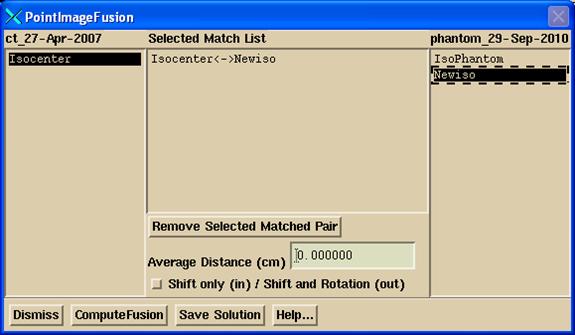
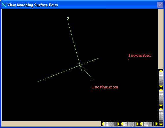
A
second contain a 3d view of the points from each image set that are selected as
matched pairs:
The
third popup has manual controls for you to get a good starting solution:
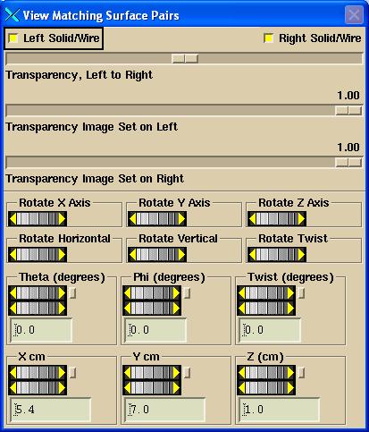
You
have two options provided with the “Shift Only” toggle button shown above in
the first pop up. If you are only
solving for shift along the x, y, and z axis, then select the toggle button
IN. You only need one matched pair of
points to solve for a shift. An average
is computed if you select more than one matched pair. Otherwise you need at least three points
matched up to also solve for rotations.
You do not need a good starting solution if solving for a shift only as
the computation is very simple. The
average distance along each of the x, y, and z axes is computed between the
matched pairs of points.
After
selecting points to match from each image set, hit the Compute Fusion button to
compute a transformation between the two image sets. The average distance between the points will
be shown after the solution and should be small of the order of 1 or 2
millimeters. The points drawn from the
image set on the left side of the list popup will be moved using the solution
to be drawn in the coordinate system of the second image set.
If
the solution fails, you may want to first try to align the two sets of points
with the rotation and translation controls provided to provide a close starting
solution. The image set on the left in
the list popup is moved to align with that on the right. The horizontal, vertical, and twist rotations
will probably be the most useful. Use
the rotation and translation tools to move image set 1 to correspond to image
set 2. Horizontal rotates around the
horizontal of the image display, vertical around the vertical, and twist around
your line of sight. Those controls are
analogous to the controls you have on the display itself. You can also rotate around the x, y, and z
axes, or specify the angles in terms of the spherical coordinates.
Fuse with Stereotactic Frames
This
is the simplest to use and probably the most accurate method to achieve image
fusion. But the frame must have been in each
image set in the same position on the patient.
The stereotactic frame must be first located on each image set. Do this under Stereotactic Frame under
Options under Stacked Image Set from the main tool bar and as described above
under Stereotactic Frames. As we noted
above:
The
stereotactic frame used in each image set must define the same anatomy. This means that the frames, if not the same
frame, are placed on the patient in the same position and the anatomy will have
the same stereotactic coordinates in each image set. Only the user of this software can determine
if these conditions are met for each case.
Other
than that, one just selects this method and the solution is computed.
Matching
Surfaces
This
method is probably the less accurate and more prone to error method than either
of the two methods described above. If
the patient is to be scanned sequentially with two imaging modalities, than you
should plan on using either a common stereotactic frame of some sort, or create
external points that will be common to both image modalities. For using common points and CT to MRI for
example, you will need some small external markers that can mark points on the
skin and will show up on both CT and MRI.
The more such markers you use the more reliable will be the
solution. A minimum of three is needed
but you should plan on more than that, six to eight. However, if you did not have control of the
imaging process you can still use internal points if they can be defined.
Matching
surfaces remains a final option for solving for image fusion. You will get three popups like you did for
the matching points method. On one popup
will be a list of all isosurfaces and outlined volumes for each image set. You will then sequentially choose
corresponding items to match up. On the
list outlined volumes are prefixed with OUT-, and isosurface volumes are
prefixed with ISOS-. You can match an
outlined volume to an isosurface volume, since both have a surface.
|
Select Surfaces to Match Tool Popup |
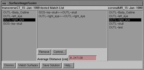
Click
the mouse on an item on the left stacked image set, and then select the
corresponding item from the list on the right for the second stacked image set.
If
you want to remove a line in the middle matched surface list, select that line
by clicking the mouse on it and hit the Remove button.
You
may specify more than one pair of structures to match.
Note
that you can match a surface from one list to two separate items on the other
list. You are responsible for making sure
that makes logical sense. For instance
you might have the complete surface in one stacked image set and two separate
pieces of the matching structure in the other stacked image set.
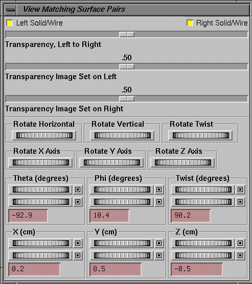
When
you have completed the list of matched structures, you should attempt to rotate
one set to align with the other. The
results of your manipulations will be visible in the popup room view
provided. The starting solution should
be close for the matching algorithm to work.
The image set on the left in the list popup is moved to align with that
on the right. The horizontal, vertical,
and twist rotations will probably be the most useful. Rotate image set 1 to correspond to image set
2. Horizontal rotates around the
horizontal of the image display, vertical around the vertical, and twist around
your line of sight. Those controls are
analogous to the controls you have on the display itself. You can also rotate around the x, y, and z
axes, or specify the angles in terms of the spherical coordinates.
|
The rotation and translation control for alligning two image sets. |
When
done aligning the two image sets, hit the Match Surfaces button to perform the
fusion process between the two stacked image sets. The transformation will be searched for that
minimizes the distances between the two surfaces. One surface is left in tact, the default is
to pick the surface with the larger number of triangles. Points are selected from the other
surface. The closest distance from each
point to the surface is measured and summed for all points. The transformation that minimizes this sum is
searched for. A down hill search method
is used for the search engine.
You
can override the program defaults for each matched pair by clicking on the
matched pair in the middle scrolled list, and hit the control button. Normally, there would be no reason to
override the defaults except that you may want to select to use more points or
force selection of which image set provides the surface and which the points.
As
an alternative you can hit the Save Solution after only manual alignment of the
two image sets, as described below.
Control for Matched Surfaces
|
Control for a matched pair of surfaces |
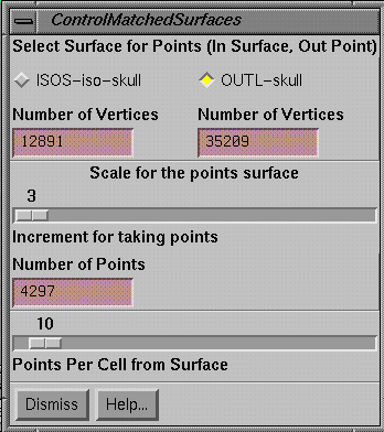
Hitting
the control button for a selected match pair brings up a fourth popup. On this control defaults for the selected
matched pair may be changed.
Select Surface Control
One
surface remains a surface defined by a collection of triangles, and the other
surface is defined only by points taken from the list of vertices. The surface with the greater number of
triangles is taken as the default to remain the surface. You may override this default by selecting
the other surface with the toggle button provided. Shown below each surface will be the number
of vertices for that surface (the number of triangles is typically 1.5 to 2.0
times the number of vertices). Each
vertex is unique, they are not repeated in the list.
Number of Points
Solution
times are smaller for the smaller number of points used from the other
surface. For the surface which is
reduced to points, the slider controls the number of points used. A value of 1 results in all the points being
used. A value of 2 results in every
other point being used, and so forth.
The bottom text field is simply the number of vertices divided by the
increment, and is the number of points that will be used to compute the
distance to the surface. The average
distance is than reported when the down hill solution algorithm is run.
Points per Cell from Surface
The
surface is divided into cells of size 1/2 cm for small volumes and 1 cm for
larger volumes. The vertices of the
surface are sorted into the respective cells that they are in. Given a point from the other surface, the
cell is found that the point lies in.
The number in the slider controls how many points in the cell will be
consulted to find the minimum distance.
The default is 10. If there are
10 or less points in the cell all points in the cell are compared to the point
from the other surface and the point which is closest is reported as the
minimum distance to the surface. If
there are more than 10 points in the cell than some points are skipped so that
the distance is computed to only 10 points, with the smallest distance being
taken. The more points per cell that is
checked, the longer the solution time.
Most likely there will not be more than 10 points per cell. Notice also that the distance to the surface
is approximated from the distance to the vertices of the triangles that make up
the surface and not to the triangle surface enclosed by the vertices. Computing the distance to each triangle that
falls inside the cell would greatly increase the solution time given the large
number of points and triangles. Because
of the large number of points, we can expect any resolution error from this
approximation to average out. This part
of the method differs from the below reference.
Reference
For
more information on these concepts see:
"Automatic
three-dimensional correlation of
An Example: CT head to MRI head
For
CT scans simply make an isosurface. The
default bone value should give a good skull but you might want to play with
that value some. A problem may arise if
the patient had a stereotactic frame. To
get rid of the frame make a body outline (under Contouring to Contours). Edit the contours to take out any contours that
go around the stereotactic frame. Then
under the Volume pulldown on the contours toolbar, choose Make Volume from Old
and make a new volume that is larger by some small margin, such as 0.5 cm. We will use this volume to restrict the
isosurface to be within. The reason for
adding a margin to the body outline is that skull goes quite close to the skin
and if we used the body outlines directly we will eliminate some skull. Generate the isosurface restricting the
isosurface to what is inside the body outline with margin.
To
generate a skull from MRI images, go under Contouring to contours. Use the Auto Contour Screen tool. Pick an image in the MRI image set and use
the Contrast tool to reverse the contrast of the MRI image. Adjust the contrast window width and center
to make the black hole where the skull was (now white since we reversed
contrast) to look as much like the skull in CT as possible. Be sure not to create other anatomy that is
not bone, such as the air cavities in the sinus. You will have to compromise here. Choose to keep inside contours on the Auto
Screen Contour tool so you won’t also pick up the body outline, and hit the
Apply to Frame to see what you get. When
satisfied that you have isolated the bone as much as possible, hit Apply to All
Frames in Screen button on the Auto Screen Contouring tool to repeat the
operation automatically on all images of the MRI image set. Be sure to hit Accept Contour before
dismissing the tool. You should be able
to generate a skull from this procedure from the MRI images.
Match
the isosurface skull from CT with the outlined skull from MRI. You might also want to outline other
structures such as the eyes to be matched up as well. The more corresponding surfaces you can
create the better. You should then
manually align the two image sets before attempting the auto algorithm.
Verification of Image Fusion
After
saving a solution for the transformation between two image sets you must verify
the solution.
First
generate two side by side images of the same plane. You may want to do this in more than one
location. Create a new screen with at
least 2 frames across the top of the screen.
Use the Copy Move Image Plane under the Stacked Image Set pulldown on
the main toolbar to select the plane from an existing image that is displayed
for one of the image sets. Deposit this
image in an empty frame. Use the Copy
Move Image Plane popup to select the other image set and deposit that image
next to the first in an empty frame.
We
would suggest that you adjust the contrast of the two images thus created to
bring out the anatomy that is most likely to help in accessing the goodness of
the fusion solution. If is easier to
adjust the contrast before using one of the two below compare tools, but you
can adjust the contrast of each image separately with either of those two tools
as well.
CT to CT
Under
Images on the main toolbar use the Compare Images - Color Mix tool. Places where the image data does not
correspond will show as a color.
CT to MRI
Under
Images on the main toolbar use the Compare Images - Checkerboard tool. You can adjust the size and spacing of the
checkerboard pattern to access how well the image data corresponds.
Image Fusion Options
Two
options exist on the image fusion options toolbar. This toolbar is found under the Stacked Image
Sets pulldown.
Display Equivalent Planes
|
Image Fusion Options Toolbar and the Display Equivalent Planes Popup
Tool |
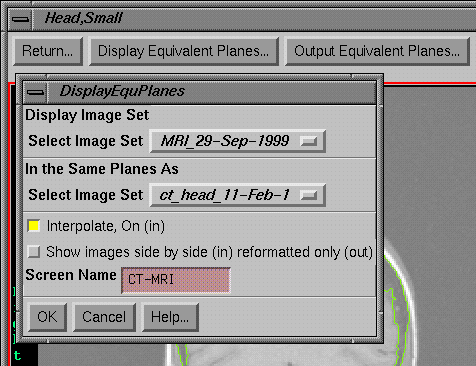
Here
one image set can be reformatted to display in the planes defined by the images
in the other image set. For every image
in the copy from image set, an image will be reformatted in the image set
selected to be displayed, regardless if that plane intersects the displayed
image set. An option also exist to
display these equivalent planes side by side with the image data coming from
one and then the other image set. In
either case a new screen is created. For
side by side images, the plane area will be the larger of the areas that
intersect each image set. For only
showing the reformatted image set, the plane size will be large enough to show
all of thedisplayed image set.
Output Equivalent Planes.
|
Image Fusion Options Toolbar and the Output Equivalent Planes Popup
Tool |
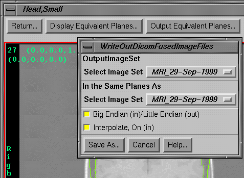
Selecting
this option will cause the image set selected for output to be reformatted and
written out in Dicom 3 format to correspond to the planes defined by another
fused image set. Like the display option
immediately above, each plane of the other image set is copied and image data
in the selected output image set is reformatted regardless of whether the plane
actually intersects the image set.
Plane Area
The
plane area will be defined by the image set supplying the image plane definitions,
the copy from image set. The plane
coordinates will also be that of the copy from image set. Therefore the files will show the same
coordinate system for the imaging system in the copy from image set, and pixel
data from the other image set is simply substituted. However, the pixel size and hence image size
may be different but the image area will be the same area (within the
resolution of one pixel).
Directory and File Name
The
user must select a directory to write these image files to and specify a file
name. Normally a new directory should be
created to hold the image files. The
directory is outside of the patient directory since these files are for export. The files will have a comma and image number
appended for each file that is written.
Byte Order
The
user must also choose whether the output files are to be Little Endian or Big
Endian. By default the program will pick
the byte order that your computer is using.
Consider the integer number 1 which is stored in four bytes. Big Endian would store this number as: 00 00 00 01, most significant byte first,
whereas Little Endian would store the bytes in reverse order: 01 00 00 00, least significant byte first,
where we list the first byte first in the order that they appear in memory.
This
program can read Dicom files written with either byte order, but other systems
might not have the flexibility. The
Dicom Standard seems to prefer Little Endian but that might not apply. We suggest you use the default unless you
discover the need for changing it.
Interpolation
As
you are reformatting images, interpolation may be performed between
slices. The default is on and you would
normally have no reason to turn it off.
Dicom Specifics
The
Dicom file header specified in PS 3.10 is not appended to the files written
out. Programs developed before this
standard would not be able to read these files.
Hopefully, programs written aftewards would be able to read files with
or without the header as this program can.
Specific Dicom
Tags
The
image type (8,8) will be: DERIVED\SECONDARY\REFORMATTED\FROMFUSION
The
instance creation date and time will be when the data is reformatted and the
file is written out.
The
SOP Instance UID (unique identifier)
will consist of 1.2.840 followed by our company ANSI number, followed by
the serial number of your computer, followed by the process ID (when the
program was running), followed by the year, month, day, hour, min, second, and
count within the second for each image file written out.
The
study and series date, times, and UID's for the same will come from a file in
the image set that the pixel data came from.
However, the coordinates for the image will come from the other image
set. This is so that the source of the
pixel data can be identified, but the image would be located relative to the
image system from which the plane definitions were taken.
All
data except as noted below will from the image set providing the pixel
data. This includes the manufacturer's
name, patient name, patient ID, and any other names. Slice thickness and slice spacing will also
come from the image set providing the pixel data.
This
computer and software will define the secondary capture device tags (18,1010),
(18,1012), (18,1014), (18,1016), (18,1018), and (18,1019) which will also
define this system that reformatted the images.
Source of Data
The
image set providing the plane definitions will provide the data for the
following tags:
(20,20),
Patient Orientation (marks edge of image left, right, superior, inferior).
(20,32),
Image Position. This is the coordinates
of the upper left hand corner of the image.
(20,37),
Image Orientation. This is the vectors
defining in patient space the horizontal and vertical directions of the image.
Data
coming from this program are tags:
(8,8),
(8,12), (8,14), (8,16), (8,23), (8,33), (8,64), (18,1010), (18,1012),
(18,1014), (18,1016), (18,1018), (18,1019), (20,13) image number, (28,2),
(28,4), (28,10), (28,11), (28,30), (28,100), (28,101), (28,102), (28,103),
(28,106), (28,107), (28,1052), (28,1053)
All
other date comes from the image set providing the pixel values.
You
can use the program DicomDump to view data in a Dicom file. The syntax is:
DicomDump
name_of _file_to_read
DicomDump
will be found in either your home directory or in the directory tools.dir.