How Dosimetry Check Works

www.MathResolutions.com

Software Products for the Radiological Sciences

Search

Home Page

Product Review

Program Manuals

Download Programs

Purchase

Site Map

Dosimetry Check

MarkRT (VGRT)

RtDosePlan

System 2100

MillComp

C++ Library

How Dosimetry Check Works

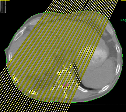
To compute the dose to the patient from a treatment portal, pencils are first created that cover the treatment field and patient. The area of a beam field is simply divided up into small pixels (in a plane perpendicular to the beam), each pixel being a separate pencil. Whether a pencil beam algorithm or a full superposition algorithm, it is necessary to trace each pencil through the patient as illustrated in the below image where we have lighted up every other pencil. Typically the density of the material the beam is going through is noted and one computes terma along each ray. However, to compute the dose to the patient one must know the intensity of radiation that reaches each ray.

In a planning system to know the intensity that is reaching each pencil on the surface of the patient, a source model is used that can compute the intensity down stream from the collimation system on any point on a plane perpendicular to the central ray, as illustrated in the below image. 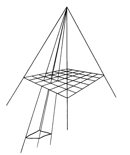The source model must take into account everything, the flattening filter, the collimator system, the multi-leaf system, wedges, and any dynamic movements of those things to arrive at the final intensity that reaches each pencil.
Dosimetry Check does not have a source model, which is the whole point of Dosimetry Check. In Dosimetry Check, the source model is replaced with a measured source model. If you were to put a piece of x-ray film on the couch and expose to the treatment portal straight down for the whole beam on time, you will have a picture of the field intensity that takes into account everything, such as leaf leakage, since you have just measured it all. In Dosimetry Check you can use the EPID or a diode or ion chamber array for greater convenience. The distance to the patient surface for each pencil is known from the CT scans and beam position.

Using x-ray film, the beam film (taken BEFORE or without the patient) gets darker the more radiation a spot gets. As noted above, the port image without the patient in the beam is a record of how much radiation each pixel gets.

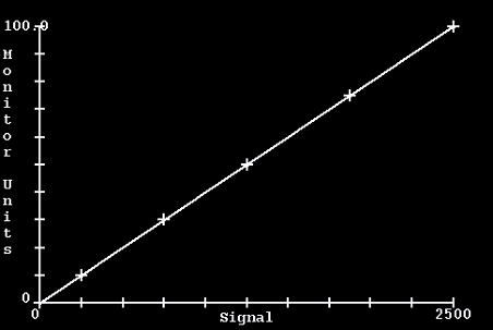
It is necessary to convert this information to a unit that will make it possible to compute the dose in centiGray to the patient from each pencil. Each spot on the image is mapped to the monitor units that would produce the same darkness at the center of a 10x10 cm field size (i.e. the field size that you calibrate the accelerator to). We call this resultant number the "relative monitor unit" (RMU). If you calibrate your machine with a 10x10 cm field size, you would use that field size to run a calibration curve. For open fields, the RMU value would be the monitor units for the beam times the scatter collimator factor for that field size. For IMRT fields, the RMU can be thought of as the effective monitor unit at that location within the radiation field. The RMU is then a measure of the in air ray field intensity, in a unit we can use directly for calculation of the dose to a phantom.

Hence we are effectively calilbrating in monitor units. To compute the dose to the patient we have to know what your definition of a monitor unit is. Some examples might be:

100 cm SSD, 10x10 cm field size, depth = 1.5 cm, 1.0 cGy/mu
or
98.5 cm SSD, 10x10 cm field size, depth = 1.5 cm, 1.0 cGy/mu
or
95 cm SSD, 10x10 cm field size, depth = 5.0 cm, 1.0 cGy/mu
or
100 cm SSD, 10x10 cm field size, depth = 10.0 cm, 0.670 cGy/mu

Basically, what ever field size you set, SSD, depth, and dose you measure per monitor unit when you check the output of your linac would be your monitor unit definition. This definition has to be specified in your beam data in Dosimetry Check.

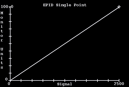
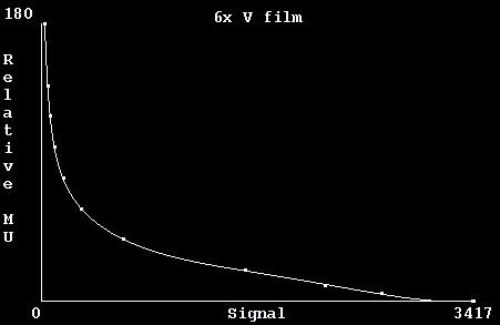To accomplish this mapping you must run a calibration curve of the pixel value at the center of a 10x10 cm field versus monitor units.

This curve is used to map the pivel values on the beam images to RMU.

Once converted to RMU, Dosimetry Check can compute the dose from a beam to the patient in centiGray. 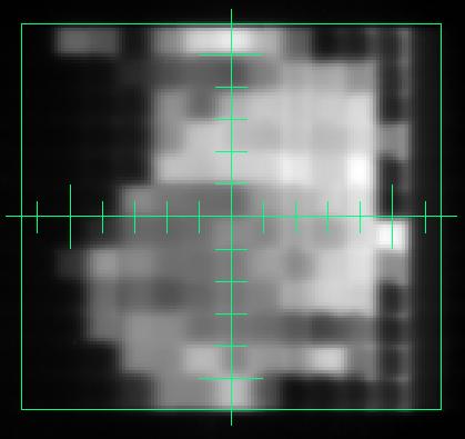Here, zero RMU is black, whiter is larger RMU.

However, for an EPID, ion chamber or diode array, integration is a linear process with zero intercept. So only one point would be needed to define the calibration curve, i.e., a straight line that goes through zero.

So one can use a single measurement of your calibration field, typically a 10x10 cm field, to determine the calibration line. This means only one 10x10 field need be measured with a clinical case to map the fluence images to RMU values, assuming zero intercept, with only one data point instead of many. If the 10x10 is exposed with 100 mu, and the signal value on the central axis of the 10x10 is S, then every pixel in the clinical image is multiplied by 100/S. You could measure the RMU value with an ion chamber, for example. Measure the point in space for the IMRT field and get reading D. Then move the chamber to the central axis, same distance, and measure S for 100 mu. The rmu is then D X 100 / S. From this it is obvious that for open fields on the central axis the RMU will be the mu times Sc, since Sc is also normalized to the calibration field size. The first step in processing clinical images is to normalize them with the calibration image to units of RMU. The calibration image is necessarily exposed with nothing in the beam.

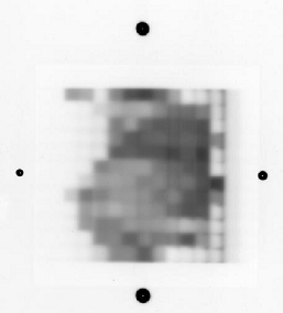
But an EPID or similar device will generate internal scatter within the device. This is corrected for by doing a deconvolution with the spread function of the device to arrive at in air fluence in RMU. Shown below is an EPID image of a modulated field for a head and neck case after mapping to RMU units (where white is more radiation).

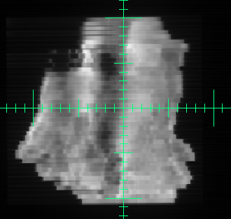
The pixels on the RMU image are used as "weights" for the corresponding pencil beams. The fluence map that we have derived here from a calibrated image of the beam completely determines the dose to the patient. This process is similiar to how a planning system computes the dose, except here we are using the measured fluence instead of computing the same from knowledge and models of what kind of things modulate the beam. By starting with measurement instead of a model, we verify the dose and dose distribution that the patient receives.

The dose computed by Dosimetry Check may be compared directly to that computed by the planning system. ADAC IMRT plan (green) versus Dosimetry Check (magenta) with inhomogeneity corrections on, courtsey of Dr. Tianyou Xue.

Transit Dosimetry with Exit Images

For transit dosimetry with exit images (beams integrated during treatment on the exit side of the patient) read the following white paper. A summary is this. The exit images are first converted to RMU as above (which we will call the raw RMU values). The pixel values are corrected for the computed path from the radiation source to the exit image. That step requires ray tracing through the CT scan set and should include a model of the treatment couch. A point spread that is a function of both radius and water equivalent thickness of what is in the beam is used to convert to in air fluence (in RMU) before the patient. The dose is then computed as above for pre-treatment images.
White paper on exit to transit dosimetry.

Return to prior page.